Data
# Libraries
library(dplyr)
library(expss) # for apply_labels
library(likert)
library(stringr)
library(scales)

# Creation of dataset
sample_prob <- function(n){
  x <- sample(1:100,n)
  return(x/sum(x))
}

set.seed(1806)
n <- 11

dataset <- data.frame(
  question1 = factor(sample(0:(n-1), size=500, replace=T, prob = sample_prob(n))),
  question2 = factor(sample(0:(n-1), size=500, replace=T, prob = sample_prob(n))),
  question3 = factor(sample(0:(n-1), size=500, replace=T, prob = sample_prob(n))),
  group = factor(sample(c("group1", "group2"), size=500, replace=T))) %>%
  apply_labels(
    question1 = "Voici un très long ou très long énoncé pour la question 1",
    question2 = "Voici un très long ou très long énoncé pour la question 2",
    question3 = "Voici un très long ou très long énoncé pour la question 3")
Basic likert plot
# Create likert object
p <- likert(dataset[, -which(names(dataset)=="group")])

# Build plot
plot(p, text.size = 4) + # text.size : size of percentage
  ggtitle("Percentage of response to questions") +
  scale_x_discrete(labels = function(x) str_wrap(x, 20)) + # if no labels, to set the width of y-axis text
  egg::theme_article() +
  theme(
    # axes
    axis.title.x = element_text(size = 8), # x axis title
    axis.text.x = element_text(size = 9), # x axis labels
    axis.title.y = element_text(size = 8), # y axis title
    axis.text.y = element_text(size = 11), # y axis labels
    # legend
    # legend.title = element_text(size = 10),
    legend.title = element_blank(),
    legend.text = element_text(size = 7.5),
    legend.position = "bottom"
  ) +
  guides(fill=guide_legend(ncol=11))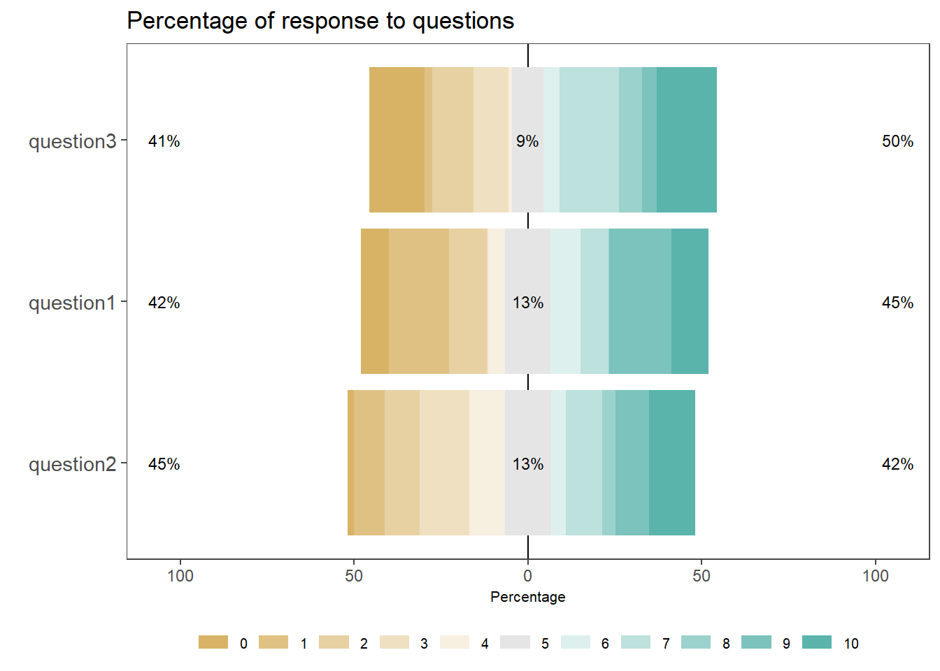
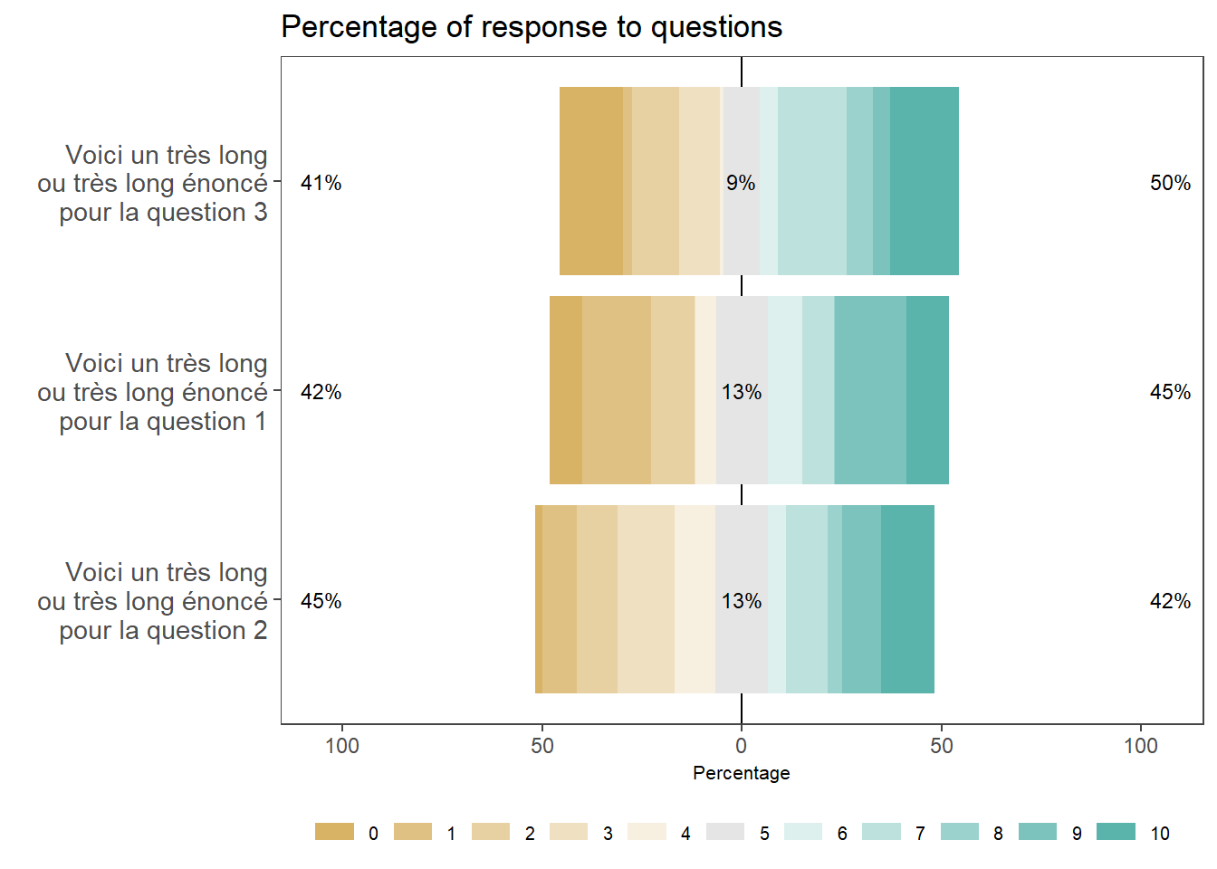
If you want to add labels:
# Function to get labels et set the width
get_label_df <- function(dataset, wrap=NULL){
  vect_label <- NULL
  for(i in names(dataset)){
    label <- attr(dataset[, i], "label")
    if(is.null(label)) label <- i
    vect_label <- c(vect_label, label)
  }
  if(!is.null(wrap)){
    vect_label <- vect_label %>% str_wrap(20)
  }
  names(vect_label) <- names(dataset)
  return(vect_label)
}

# Create likert object
p <- likert(dataset[, -which(names(dataset)=="group")])

# Label vector with wrap option to set the width of the y-axis text
vect_labels <- get_label_df(p$items, 20)

# Build plot
plot(p, size = 3) + # text.size : size of percentage
  ggtitle("Percentage of response to questions") +
  # scale_x_discrete(labels = function(x) str_wrap(x, 20)) + # if no labels, to set the width of y-axis text
  scale_x_discrete(labels = vect_labels) +
  egg::theme_article() +
  theme(
    # axes
    axis.title.x = element_text(size = 8), # x axis title
    axis.text.x = element_text(size = 9), # x axis labels
    axis.title.y = element_text(size = 8), # y axis title
    axis.text.y = element_text(size = 11), # y axis labels
    # legend
    # legend.title = element_text(size = 10),
    legend.title = element_blank(),
    legend.text = element_text(size = 7.5),
    legend.position = "bottom"
  ) +
  guides(fill=guide_legend(ncol=11))