We will here use the dessin_forest_simple function in
the Data & Functions
page.
Download Forest_autom.R
# Libraries
library(forestplot) # version 3.1.1
library(tidyverse)
library(conflicted)
conflict_prefer("filter", "dplyr")
conflict_prefer("select", "dplyr")

# Creation of dataset
set.seed(1234)

variable <- paste0("var", 1:7)

est1_mean <- rexp(7, 1)
est1_var <- rexp(7, 8)
est1_lower = est1_mean-1.96*sqrt(est1_var)
est1_upper = est1_mean+1.96*sqrt(est1_var)

est2_mean <- rexp(7, 2)
est2_var <- rexp(7, 10)
est2_lower = est2_mean-1.96*sqrt(est2_var)
est2_upper = est2_mean+1.96*sqrt(est2_var)

est3_mean <- rexp(7, 3)
est3_var <- rexp(7, 10)
est3_lower = est3_mean-1.96*sqrt(est3_var)
est3_upper = est3_mean+1.96*sqrt(est3_var)

base_data <- data.frame(variable,
                        est1_mean, est1_lower, est1_upper,
                        est2_mean, est2_lower, est2_upper,
                        est3_mean, est3_lower, est3_upper)
head(base_data)
base_data_long <- base_data %>%
pivot_longer(
!c(variable),
names_to = c("estimator", ".value"),
names_sep = "_"
)
head(base_data_long)# we set an order according to a variable
base_data_long_forest <- base_data_long %>%
left_join(base_data_long %>%
filter(estimator=="est1") %>%
arrange(mean) %>%
mutate(order = 1:n()) %>%
select(variable, order))dessin_forest_simple function
Arguments
dessin_forest_simple(
data_frame,
database with variable, mean, lower, upper columns.
name_col_var = "Variable", desired column name with
variables.
name_col_mean = "HR (95%CI)", desired
column name with estimates.
zero = 1, where we want to
put the zero of the forest plot.
pos_graphique = 3,
can be equal to 1, 2, 3 or 4, localisation of the graph
print_mean = TRUE, FALSE: remove the column with the
estimate
IC = TRUE, TRUE: displays the CI in the
column with the estimate.
boxsize = NULL, Override the
default box size based on precision
digit = 2, to
round off the estimate and its confidence interval.
lwd.ci = 1, confidence interval thickness.
clip, allows to choose the upper and lower limits of the
x-axis.
- by default: from minimum HR/OR to maximum HR/OR
- we specify the limits: vector of size 2 with the lower
bound and the upper bound
- “clip_tot”: we display the
whole graph
by = 0.5, allows to choose the distance
between the different ticks of the x-axis.
print_pval = FALSE TRUE : print the pvalue in the last
column
new_page = TRUE TRUE : If you want the plot to
appear on a new blank page
favors, vector with the
names to display below axis for directional difference (optional)
favors_fontsize = 15, fontsize for the text display below
axis for directional difference
y_favors_arrow,
coordinate for favors arrows (optional)
y_favors_text,
coordinate for favors labels (optional)
)
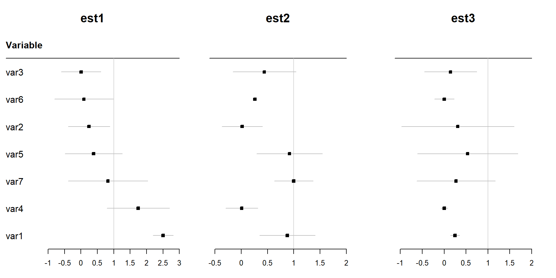
fp1 <- dessin_forest_simple(base_data_long_forest %>% filter(estimator=="est1") %>% arrange(order), print_mean=FALSE,
                            boxsize=0.1, clip="clip_tot",
                            name_col_mean = "est1",
                            print_variable=TRUE)
fp2 <- dessin_forest_simple(base_data_long_forest %>% filter(estimator=="est2") %>% arrange(order), print_mean=FALSE,
                            boxsize=0.1, clip="clip_tot",
                            name_col_mean = "est2",
                            print_variable=FALSE,
                            new_page = FALSE)
fp3 <- dessin_forest_simple(base_data_long_forest %>% filter(estimator=="est3") %>% arrange(order), print_mean=FALSE,
                            boxsize=0.1, clip="clip_tot",
                            name_col_mean = "est3",
                            print_variable=FALSE,
                            new_page = FALSE)

grid.newpage()
pushViewport(viewport(layout = grid.layout(1, 3)))

pushViewport(viewport(layout.pos.col = 1))
plot(fp1)
popViewport(1)

pushViewport(viewport(layout.pos.col = 2))
plot(fp2)
popViewport(1)

pushViewport(viewport(layout.pos.col = 3))
plot(fp3)
popViewport(1)