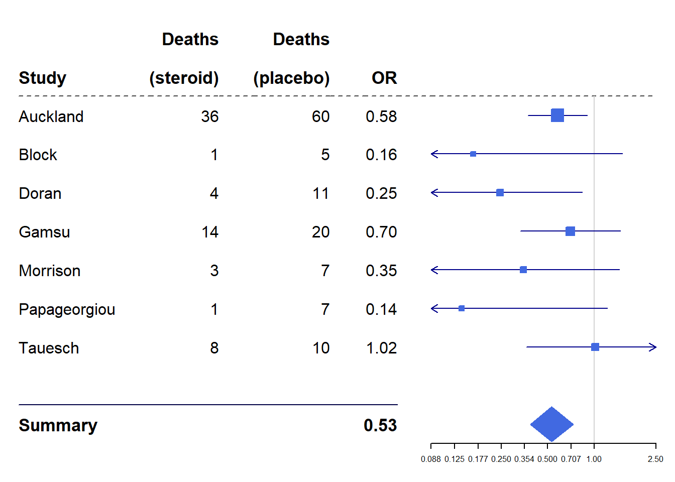
Tips to read

each line corresponds to a study
the symbol (here square or diamond) corresponds to the estimate of the parameter studied (here a relative risk)
the size of the symbol is proportional to the precision
the vertical bar is the value of the parameter in the absence of effect (here 1 because it is a relative risk)
the horizontal bars correspond to the confidence interval of the reported parameter (here the relative risk)
if the symbol is on the right of the vertical line, it means that the link between the treatment (here inspiratory muscle training) and the endpoint (here survival) is positive
if the symbol is to the left of the vertical line, it means that the link between the treatment (here inspiratory muscle training) and the endpoint (here survival) is negative
if the horizontal bar crosses the vertical bar then the link is not significant
the diamond represents the parameter estimated from all the studies

Meta-analysis forest plot

# Libraries
library(forestplot)
library(tibble)
library(tidyjson)
library(dplyr)

# Cochrane data
base_data <- tibble(mean  = c(0.578, 0.165, 0.246, 0.700, 0.348, 0.139, 1.017), 
                    lower = c(0.372, 0.018, 0.072, 0.333, 0.083, 0.016, 0.365),
                    upper = c(0.898, 1.517, 0.833, 1.474, 1.455, 1.209, 2.831),
                    study = c("Auckland", "Block", "Doran", "Gamsu", "Morrison", "Papageorgiou", "Tauesch"),
                    deaths_steroid = c("36", "1", "4", "14", "3", "1", "8"),
                    deaths_placebo = c("60", "5", "11", "20", "7", "7", "10"),
                    OR = c("0.58", "0.16", "0.25", "0.70", "0.35", "0.14", "1.02"))

summary <- tibble(mean  = 0.531, 
                  lower = 0.386,
                  upper = 0.731,
                  study = "Summary",
                  OR = "0.53",
                  summary = TRUE)

header <- tibble(study = c("", "Study"),
                 deaths_steroid = c("Deaths", "(steroid)"),
                 deaths_placebo = c("Deaths", "(placebo)"),
                 OR = c("", "OR"),
                 summary = TRUE)

empty_row <- tibble(mean = NA_real_)

cochrane_output_df <- bind_rows(header,
                                base_data,
                                empty_row,
                                summary)

cochrane_output_df %>% 
  forestplot(labeltext = c(study, deaths_steroid, deaths_placebo, OR), 
             is.summary = summary,
             clip = c(0.1, 2.5), 
             hrzl_lines = list("3" = gpar(lty = 2), 
                               "11" = gpar(lwd = 1, columns = 1:4, col = "#000044")),
             xlog = TRUE,
             col = fpColors(box = "royalblue",
                            line = "darkblue", 
                            summary = "royalblue",
                            hrz_lines = "#444444"))

Contact

This document is a work of the statistics team in the Biostatistics and Medical Information Department at Saint-Louis Hospital in Paris (SBIM).
Developed and updated by Noémie Bigot and Anouk Walter-Petrich
noemie.bigot@aphp.fr; anouk.walter-petrich@u-paris.fr

Based on The R Graph Gallery by Yan Holtz.

SBIM