We will here use the ggcompetingrisks1 and the
ggcombine functions in the Data & Functions
page.
Download
ggcompetingrisks1.R
# Libraries
library(cmprsk)
library(survminer)
library(ggplot2)

# Creation of dataset
set.seed(2)
df <- data.frame(event=sample(c(0, 1),100,replace=TRUE,prob = c(0.4, 0.6)), del_event=rexp(100)*5,
                 deces=sample(c(0, 1),100,replace=TRUE,prob = c(0.1, 0.9)), del=rexp(100)*10,
                 group=sample(c("A", "B"),100,replace=TRUE))
head(df)df$event_surv <- df$event
df$event <- ifelse(df$event==1, 1, ifelse(df$deces==1, 2, 0))
df$del_event[df$event==0] <- df$del[df$event==0]
df$del[!is.na(df$del_event) & df$del_event>df$del] <- df$del_event[!is.na(df$del_event) & df$del_event>df$del]
df$EFS <- ifelse(df$event==1 | df$deces==1, 1, 0)
df$del_EFS <- pmin(df$del, df$del_event, na.rm=T)
# cuminc object
fit <- cuminc(df$del_event, df$event)
# surv objet
fit_event_surv <- survfit(Surv(del_event, event_surv)~1, data=df)
fit_OS <- survfit(Surv(del, deces)~1, data=df)
fit_EFS <- survfit(Surv(del_EFS, EFS)~1, data=df)Create all plots:
# We set the xlim, break time
break.time.by <- 6
xlim <- c(0, 24)

#icc
var_time <- "del_event"
palette <- "#00BA38"

plot.icc <- ggcompetingrisks1(
  fit,
  xlab = "Time (months)", ylab="Cumulative incidence",
  xlim=xlim, ylim=c(0, 1),
  lwd=0.5,
  title="", legend="none", legend.title="",
  palette=palette,
  conf.int = F,
  event_suppr = c(2),
  ggtheme = theme_classic(),
) + scale_x_continuous(breaks = seq(0, floor(max(df[, var_time], na.rm=T)), break.time.by))


num.icc <- ggrisktable(
  fit_event_surv,
  data=df,
  xlim=xlim,
  break.time.by = break.time.by,
  # color = palette,                   # whole line of number at risk in color
  y.text = TRUE,
  y.text.col = palette,
  legend.labs=c(""),
  fontsize=3,
  tables.theme = theme_cleantable())    +
  theme(plot.title = element_text(size = 11, color = "black", face = "plain" ))


icc <- ggarrange(plot.icc, num.icc, ncol = 1, nrow = 2, heights = c(0.85, 0.15), align = "v")

# OS :
palette <- "#619CFF"
plot.OS <- ggsurvplot(fit_OS,
                        xlab = "Time (months)", ylab="Survival probability",
                        xlim=xlim, ylim=c(0, 1),
                        lwd=0.5,
                        break.time.by = break.time.by,
                        title="", legend="top", legend.title="",
                        legend.labs=c("OS"),
                        palette=palette,
                        conf.int = FALSE,
                        conf.int.fill = palette,
                        ggtheme = theme_classic(),
                        risk.table = T,
                        risk.table.y.text = TRUE,
                        risk.table.y.text.col = TRUE,
                        risk.table.fontsize=3,
                        tables.theme = theme_cleantable())

plot.OS$table <- plot.OS$table +
  theme(plot.title = element_text(size = 11, color = "black", face = "plain" ))
OS <- ggarrange(plot.OS$plot, plot.OS$table, ncol = 1, nrow = 2, heights = c(0.85, 0.15), align = "v")


# EFS :
palette <- "#F8766D"
plot.EFS <- ggsurvplot(fit_EFS,
                      xlab = "Time (months)", ylab="Survival probability",
                      xlim=xlim, ylim=c(0, 1),
                      lwd=0.5,
                      break.time.by = break.time.by,
                      title="", legend="top", legend.title="",
                      legend.labs=c("EFS"),
                      palette=palette,
                      conf.int = FALSE,
                      conf.int.fill = palette,
                      ggtheme = theme_classic(),
                      risk.table = T,
                      risk.table.y.text = TRUE,
                      risk.table.y.text.col = TRUE,
                      risk.table.fontsize=3,
                      tables.theme = theme_cleantable())

plot.EFS$table <- plot.EFS$table +
  theme(plot.title = element_blank())
EFS <- ggarrange(plot.EFS$plot, plot.EFS$table, ncol = 1, nrow = 2, heights = c(0.85, 0.15), align = "v")

ggarrange(OS, EFS, icc, ncol = 3, nrow = 1)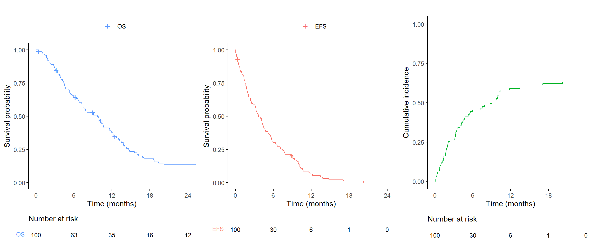
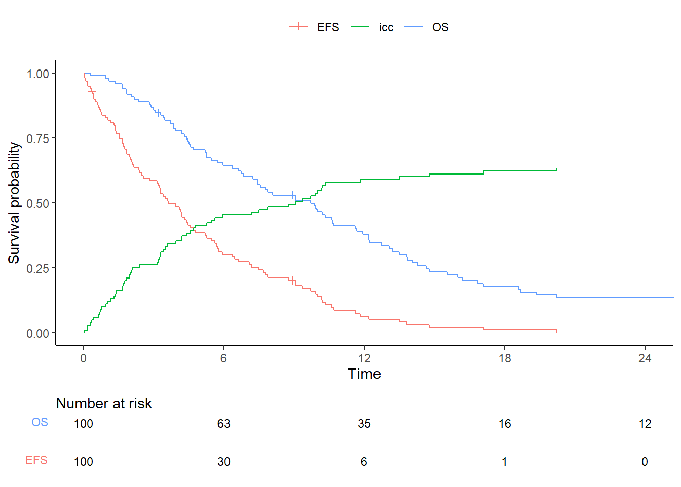
Combine ggsurvplot and ggcompetingrisks in
the same plot:
list_obj <- list(plot.OS, plot.EFS, plot.icc)
name_obj <- c("OS", "EFS", "icc")

plot.all <- ggcombine(list_obj, name_obj) +
  theme_classic() +
  theme(legend.position="top") + labs(color="") +
  xlab("Time") + ylab("Survival probability") +
  ylim(0, 1) +
  coord_cartesian(xlim = xlim) +
  scale_x_continuous(breaks = seq(0, xlim[2], break.time.by))

ggarrange(plot.all, plot.OS$table, plot.EFS$table, ncol = 1, nrow = 3, heights = c(0.8, 0.1, 0.1), align = "v")