We will here use the ggcompetingrisks1 function in the
Data & Functions
page.
Download
ggcompetingrisks1.R
# Libraries
library(cmprsk)
library(survminer)
library(ggplot2)

# Creation of dataset
set.seed(2)
df <- data.frame(del=rexp(100)*5,
                 event=sample(c(0, 1, 2),100,replace=TRUE,prob = c(0.3, 0.6, 0.1)),
                 group=sample(c("A", "B"),100,replace=TRUE))
df$event_surv <- ifelse(df$event==0, 0, 1)

# cuminc object
fit_gp <- cuminc(df$del, df$event, df$group)

# surv objet
fit_surv_gp <- survfit(Surv(del, event_surv)~group, data=df)
# !!!! warning !!!! always use survfit with "data="
You can plot with different colors, linetypes, or colors and
linetypes with the argument type_group.
Plot with different colors
Example with default colors (palette hue_pal chosen
automatically by ggcompetingrisks1, but to be fixed if you
want the same colors in ggrisktable).
# We set the xlim, break time, var_time and palette
break.time.by <- 6
var_time <- "del"
xlim <- c(0, 24)
palette <- scales::hue_pal()(2)
# palette <- c("red", "blue")

plot.icc.gp=ggcompetingrisks1(
  fit_gp,
  xlab = "Time (months)",
  xlim=xlim, ylim=c(0, 1),
  lwd=0.5,
  title="", legend="top",
  legend.title="Legend title",
  labs=c("Group A", "Group B"),
  palette=palette,
  conf.int = T,
  type_group="color",
  event_suppr = 2,
  ggtheme = theme_classic()
) + scale_x_continuous(breaks = seq(0, floor(max(df[, var_time], na.rm=T)), break.time.by)) +
  annotate(geom="text", x=1, y=0.75, label=paste0("p = ",format.pv(fit_gp$Tests[row.names(fit_gp$Tests)=="1","pv"]))) # gray's test for event 1

# !!!! warning !!!! always use survfit with "data="
num.icc.gp <- ggrisktable(
  fit_surv_gp,
  data=df,
  xlim=xlim,
  break.time.by = break.time.by,
  palette=palette,
  # color = "group",
  y.text = TRUE,
  y.text.col = palette,
  fontsize=3,
  legend="none",
  legend.labs=c("Group A", "Group B"),
  tables.theme = theme_cleantable()) +
  theme(plot.title = element_text(size = 11, color = "black", face = "plain" ))

icc.gp <- ggarrange(plot.icc.gp, num.icc.gp, ncol = 1, nrow = 2, heights = c(0.85, 0.15), align = "v")
icc.gp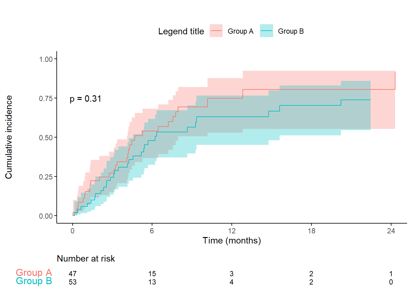
Using ggsurvplot with the same graphic parameters:
plot.surv.gp <- ggsurvplot(fit_surv_gp,
                        xlab = "Time (months)", ylab="Survival probability",
                        xlim=xlim, ylim=c(0, 1),
                        lwd=0.5,
                        break.time.by = break.time.by,
                        title="", legend="top", legend.title="Legend title",
                        legend.labs=c("Group A", "Group B"),
                        palette=palette,
                        conf.int = TRUE, pval=T, pval.size=4,
                        ggtheme = theme_classic(),
                        risk.table = T,
                        # risk.table.col = "group",
                        risk.table.y.text = TRUE,
                        risk.table.y.text.col = TRUE,
                        risk.table.fontsize=3,
                        risk.table.show.legend = FALSE,
                        tables.theme = theme_cleantable())

plot.surv.gp$table <- plot.surv.gp$table +
  theme(plot.title = element_text(size = 11, color = "black", face = "plain" ),
        text = element_text(size=15), legend.position = "none")
surv.gp <- ggarrange(plot.surv.gp$plot, plot.surv.gp$table, ncol = 1, nrow = 2, heights = c(0.85, 0.15), align = "v")
surv.gp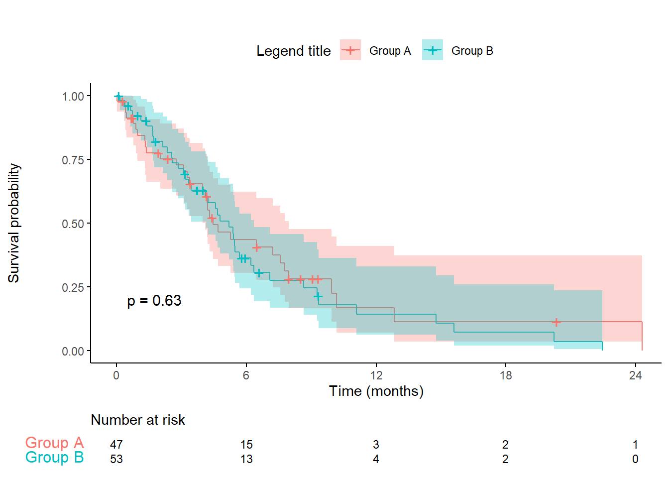
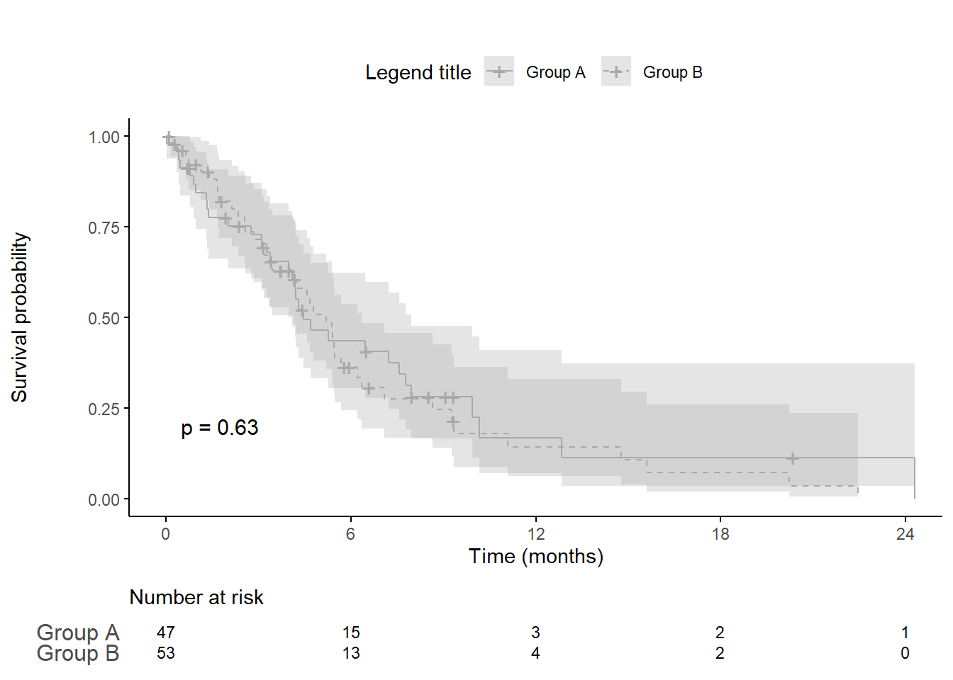
Plot with different linetypes
# We set the xlim, break time, var_time and palette
break.time.by <- 6
var_time <- "del"
xlim <- c(0, 24)
palette <- c("darkgray")

plot.icc.gp=ggcompetingrisks1(
  fit_gp,
  xlab = "Time (months)", ylab="Cumulative incidence",
  xlim=xlim, ylim=c(0, 1),
  lwd=0.5,
  title="", legend="top",
  legend.title="Legend title",
  labs=c("Group A", "Group B"),
  palette=palette,
  conf.int = T,
  type_group="linetype",
  event_suppr = 2,
  ggtheme = theme_classic()
) + scale_x_continuous(breaks = seq(0, floor(max(df[, var_time], na.rm=T)), break.time.by))+
  annotate(geom="text", x=1, y=0.75, label=paste0("p = ",format.pv(fit_gp$Tests[row.names(fit_gp$Tests)=="1","pv"]))) # gray's test for event 1

# !!!! warning !!!! always use survfit with "data="
num.icc.gp <- ggrisktable(
  fit_surv_gp,
  data=df,
  xlim=xlim,
  break.time.by = break.time.by,
  palette=c(palette, palette),
  # color = "group",
  y.text = TRUE,
  # y.text.col = palette,
  fontsize=3,
  legend="none",
  legend.labs=c("Group A", "Group B"),
  tables.theme = theme_cleantable()) +
  theme(plot.title = element_text(size = 11, color = "black", face = "plain" ))

icc.gp <- ggarrange(plot.icc.gp, num.icc.gp, ncol = 1, nrow = 2, heights = c(0.85, 0.15), align = "v")
icc.gp
Using ggsurvplot with the same graphic parameters:
plot.surv.gp <- ggsurvplot(fit_surv_gp,
                           xlab = "Time (months)", ylab="Survival probability",
                           xlim=xlim, ylim=c(0, 1),
                           lwd=0.5,
                           break.time.by = break.time.by,
                           title="", legend="top", legend.title="Legend title",
                           legend.labs=c("Group A", "Group B"),
                           palette=c(palette, palette),
                           linetype = c(1, 2),
                           conf.int = TRUE, pval=T, pval.size=4,
                           ggtheme = theme_classic(),
                           risk.table = T,
                           # risk.table.col = "group",
                           risk.table.y.text = TRUE,
                           risk.table.y.text.col = FALSE,
                           risk.table.fontsize=3,
                           risk.table.show.legend = FALSE,
                           tables.theme = theme_cleantable())

plot.surv.gp$table <- plot.surv.gp$table +
  theme(plot.title = element_text(size = 11, color = "black", face = "plain" ),
        text = element_text(size=15, color="black"), legend.position = "none")
surv.gp <- ggarrange(plot.surv.gp$plot, plot.surv.gp$table, ncol = 1, nrow = 2, heights = c(0.85, 0.15), align = "v")
surv.gp
Plot with different colors and linetypes
# We set the xlim, break time, var_time and palette
break.time.by <- 6
var_time <- "del"
xlim <- c(0, 24)
palette <- scales::hue_pal()(2)


plot.icc.gp=ggcompetingrisks1(
  fit_gp,
  xlab = "Time (months)",
  xlim=xlim, ylim=c(0, 1),
  lwd=0.5,
  title="", legend="top",
  legend.title="Legend title",
  labs=c("Group A", "Group B"),
  palette=palette,
  conf.int = T, multiple_panels = F, type_group="color_linetype",
  event_suppr = 2,
  ggtheme = theme_classic()
) + scale_x_continuous(breaks = seq(0, floor(max(df[, var_time], na.rm=T)), break.time.by))+
  annotate(geom="text", x=1, y=0.75, label=paste0("p = ",format.pv(fit_gp$Tests[row.names(fit_gp$Tests)=="1","pv"]))) # gray's test for event 1

# !!!! warning !!!! always use survfit with "data="
num.icc.gp <- ggrisktable(
  fit_surv_gp,
  data=df,
  xlim=xlim,
  break.time.by = break.time.by,
  palette=palette,
  # color = "group",
  y.text = TRUE,
  y.text.col = palette,
  fontsize=3,
  legend="none",
  legend.labs=c("Group A", "Group B"),
  tables.theme = theme_cleantable()) +
  theme(plot.title = element_text(size = 11, color = "black", face = "plain" ))

icc.gp <- ggarrange(plot.icc.gp, num.icc.gp, ncol = 1, nrow = 2, heights = c(0.85, 0.15), align = "v")
icc.gp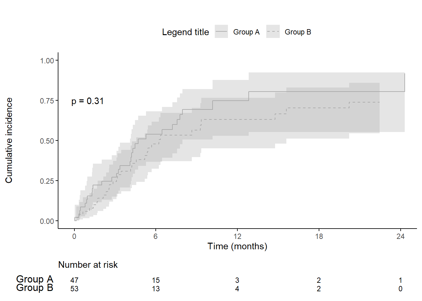
Using ggsurvplot with the same graphic parameters:
plot.surv.gp <- ggsurvplot(fit_surv_gp,
                           xlab = "Time (months)", ylab="Survival probability",
                           xlim=xlim, ylim=c(0, 1),
                           lwd=0.5,
                           break.time.by = break.time.by,
                           title="", legend="top", legend.title="Legend title",
                           legend.labs=c("Group A", "Group B"),
                           # palette=palette,
                           linetype = c(1, 2),
                           conf.int = TRUE, pval=T, pval.size=4,
                           ggtheme = theme_classic(),
                           risk.table = T,
                           # risk.table.col = "group",
                           # risk.table.y.text = TRUE,
                           risk.table.fontsize=3,
                           risk.table.show.legend = FALSE,
                           tables.theme = theme_cleantable())

plot.surv.gp$table <- plot.surv.gp$table +
  theme(plot.title = element_text(size = 11, color = "black", face = "plain" ),
        text = element_text(size=15), legend.position = "none")
surv.gp <- ggarrange(plot.surv.gp$plot, plot.surv.gp$table, ncol = 1, nrow = 2, heights = c(0.85, 0.15), align = "v")
surv.gp