Basic Competing Risks Curves

We will here use the ggcompetingrisks1 function in the Data & Functions page.
Download ggcompetingrisks1.R

# Libraries
library(cmprsk)
library(survminer)
library(ggplot2)

# Data used
set.seed(2)
df <- data.frame(del=rexp(100)*5, 
                 event=sample(c(0, 1, 2),100,replace=TRUE,prob = c(0.3, 0.6, 0.1)), 
                 group=sample(c("A", "B"),100,replace=TRUE))
df$event_surv <- ifelse(df$event==0, 0, 1)

# cuminc object 
fit <- cuminc(df$del, df$event)
# surv objet 
fit_surv <- survfit(Surv(del, event_surv)~1, data=df) # !!!! warning !!!! always use survfit with "data="

You can plot with different colors, linetypes, or colors and linetypes with the argument “type_event”.

Plot with different colors

Example with default colors (palette hue_pal chosen automatically by ggcompetingrisks1).

# We set the xlim, break time, var_time and palette
break.time.by <- 6
var_time <- "del"
xlim <- c(0, 24)
palette <- scales::hue_pal()(2)

plot.icc=ggcompetingrisks1(
  fit,                                         
  xlab = "Time (months)", ylab="Cumulative incidence",
  xlim=xlim, ylim=c(0, 1), 
  lwd=0.5,                                        
  title="", legend="top", legend.title="Event",  
  labs_event=c("event 1", "event 2"), type_event="color", 
  # palette=palette,
  conf.int = T,
  ggtheme = theme_classic(),                   
) + scale_x_continuous(breaks = seq(0, floor(max(df[, var_time], na.rm=T)), break.time.by))

# !!!! warning !!!! always use survfit with "data="
num.icc <- ggrisktable(
  fit_surv,             
  data=df,
  xlim=xlim,
  break.time.by = break.time.by,     
  y.text = TRUE,   
  legend.labs=c(""),
  fontsize=3,           
  tables.theme = theme_cleantable())    +
  theme(plot.title = element_text(size = 11, color = "black", face = "plain" )) 


icc <- ggarrange(plot.icc, num.icc, ncol = 1, nrow = 2, heights = c(0.85, 0.15), align = "v")
icc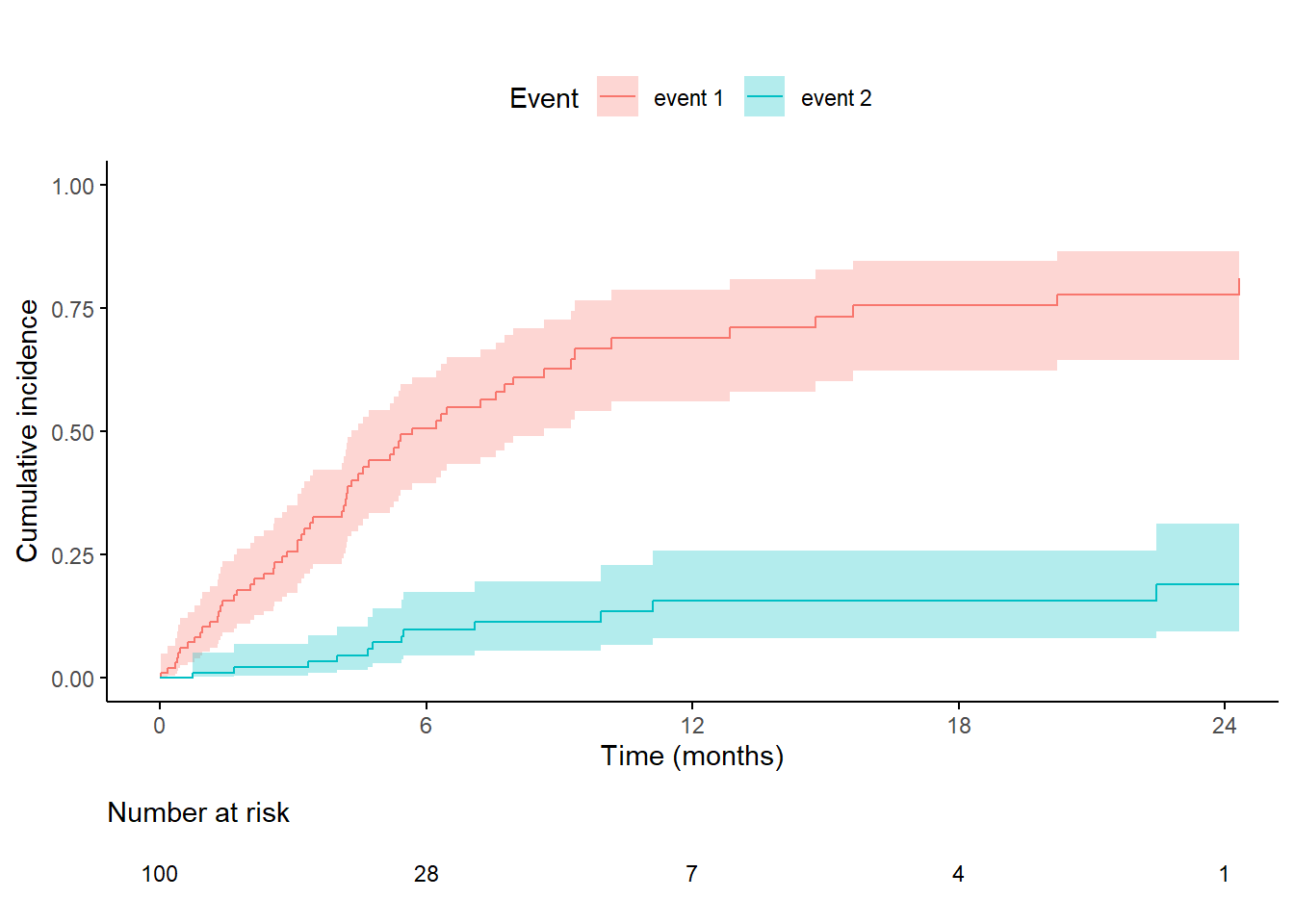

Plot with different linetypes

# We set the xlim, break time, var_time and palette
break.time.by <- 6
var_time <- "del"
xlim <- c(0, 24)
palette <- c("grey")

plot.icc=ggcompetingrisks1(
  fit,                                         
  xlab = "Time (months)", ylab="Cumulative incidence",
  xlim=xlim, ylim=c(0, 1), 
  lwd=0.5,                                        
  title="", legend="top", legend.title="Event",  
  labs_event=c("event 1", "event 2"), type_event="linetype", 
  palette=palette,
  conf.int = T,
  ggtheme = theme_classic(),                   
) + scale_x_continuous(breaks = seq(0, floor(max(df[, var_time], na.rm=T)), break.time.by))

# !!!! warning !!!! always use survfit with "data="
num.icc <- ggrisktable(
  fit_surv,             
  data=df,
  xlim=xlim,
  break.time.by = break.time.by,     
  # color = palette,               
  y.text = TRUE,       
  # y.text.col = palette,
  legend.labs=c(""),
  fontsize=3,           
  tables.theme = theme_cleantable())    +
  theme(plot.title = element_text(size = 11, color = "black", face = "plain" )) 


icc <- ggarrange(plot.icc, num.icc, ncol = 1, nrow = 2, heights = c(0.85, 0.15), align = "v")
icc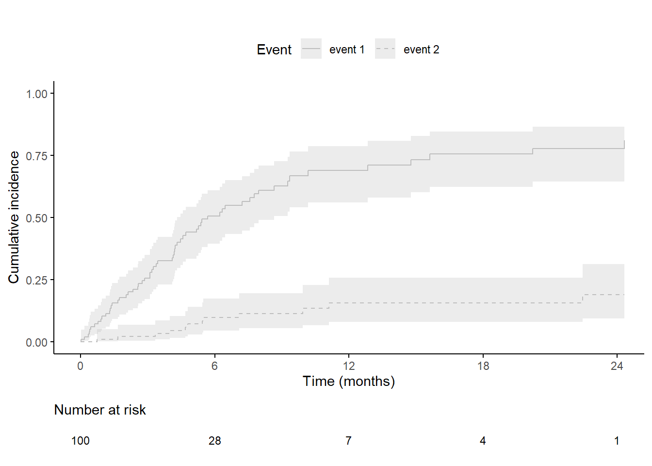

Plot with different colors and linetypes

# We set the xlim, break time, var_time and palette
break.time.by <- 6
var_time <- "del"
xlim <- c(0, 24)
palette <- scales::hue_pal()(2)

plot.icc=ggcompetingrisks1(
  fit,                                         
  xlab = "Time (months)", ylab="Cumulative incidence",
  xlim=xlim, ylim=c(0, 1), 
  lwd=0.5,                                        
  title="", legend="top", legend.title="Event",  
  labs_event=c("event 1", "event 2"), type_event="color_linetype", 
  # palette=palette,
  conf.int = T,
  ggtheme = theme_classic(),                   
) + scale_x_continuous(breaks = seq(0, floor(max(df[, var_time], na.rm=T)), break.time.by))

# !!!! warning !!!! always use survfit with "data="
num.icc <- ggrisktable(
  fit_surv,             
  data=df,
  xlim=xlim,
  break.time.by = break.time.by,     
  y.text = TRUE,       
  legend.labs=c(""),
  fontsize=3,           
  tables.theme = theme_cleantable())    +
  theme(plot.title = element_text(size = 11, color = "black", face = "plain" )) 


icc <- ggarrange(plot.icc, num.icc, ncol = 1, nrow = 2, heights = c(0.85, 0.15), align = "v")
icc

Contact

This document is a work of the statistics team in the Biostatistics and Medical Information Department at Saint-Louis Hospital in Paris (SBIM).
Based on The R Graph Gallery by Yan Holtz.

SBIM