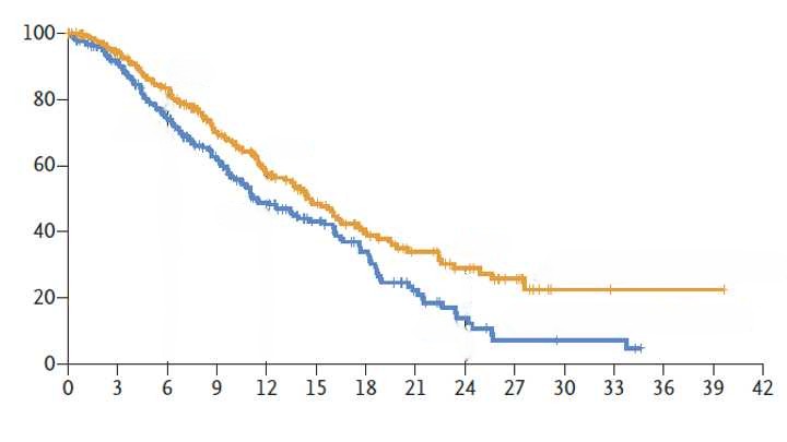
To reconstruct a Kaplan-Meier curve and generate pseudo individual patient data (IPD), several steps are required. The example below is based on the following image (Download).

Step 1: Digitization

SurvdigitizeR is an R package that automates the extraction of survival probabilities from Kaplan-Meier (KM) curves in JPEG or PNG format. It simplifies the process of digitizing KM curves, which is typically time-consuming and prone to error when done manually. This package provides an efficient and accurate way to digitize KM curves.

# Libraries
#devtools::install_github("Pechli-Lab/SurvdigitizeR")
library(SurvdigitizeR)
library(tidyverse)
library(ggplot2)


# Digitization
set.seed(1354534)
CourbSurv_time <- survival_digitize(img_path = "article_surv.jpg",
                                    x_start = 0, x_end = 42, x_increment = 3,
                                    y_start = 0, y_end = 1, y_increment = 0.2,
                                    y_text_vertical =  TRUE, # if the Y-axis labels are vertical or horizontal
                                    censoring = TRUE, # if censoring is represented by black marks
                                    line_censoring = TRUE, # if line censoring removal should be attempted
                                    num_curves = 2)

CourbSurv_time %>%
  ggplot(aes(x = time, y= St, color = as.factor(curve), group = curve)) +
  geom_step() + ylim(0,1) + theme_bw() +
  scale_x_continuous(breaks = seq(0,42,3)) +
  scale_y_continuous(breaks = seq(0,1,0.2))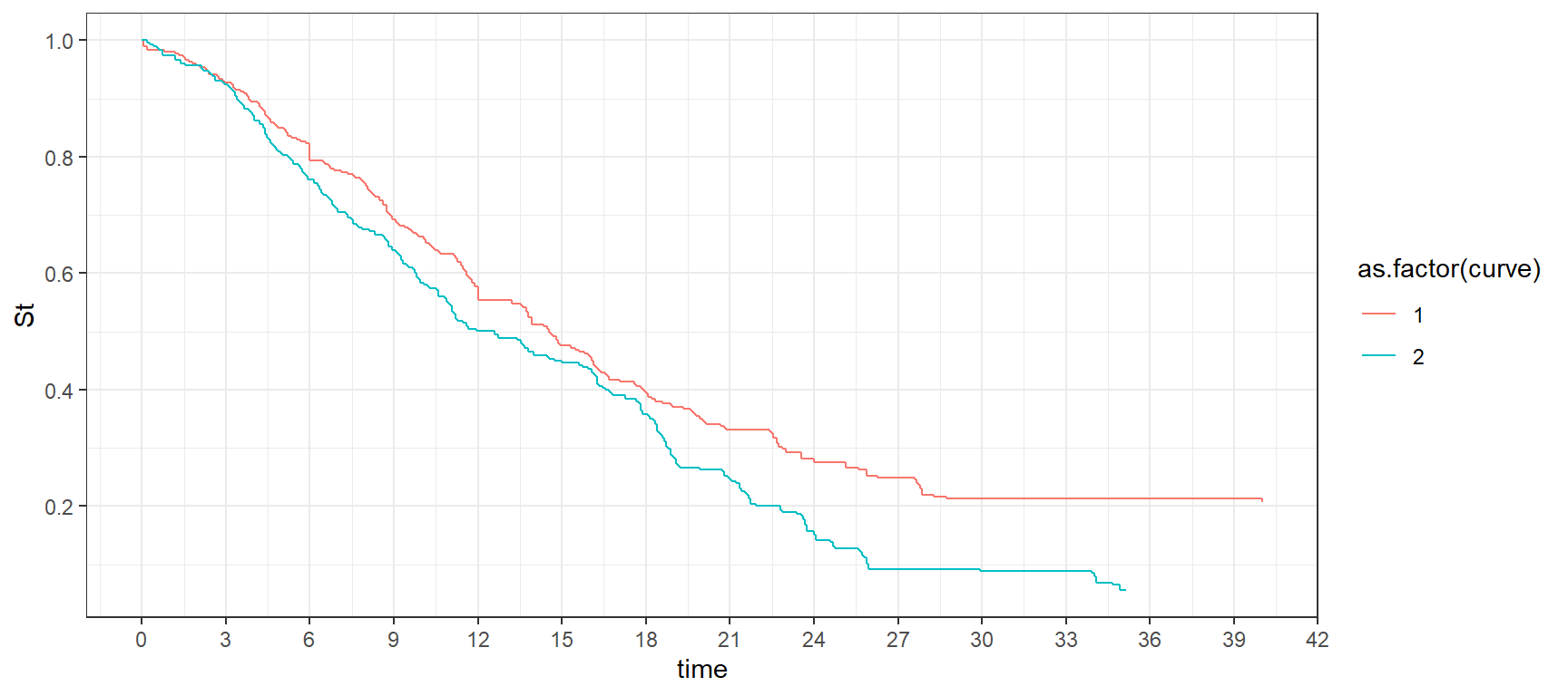

Step 2: Number at risk

In this step, the number of patients at risk at specific time points is reported. These values are used to align the digitized survival probabilities with the patient counts and improve reconstruction accuracy.

# Number at risk
N_timepoints <- 15
CourbSurv_nrisk <- data.frame(
  Group = c(rep(1,N_timepoints),rep(2,N_timepoints)), # 2 groups
  Interval = rep(1:N_timepoints,2),
  Time = rep(c(0,3,6,9,12,15,18,21,24,27,30,33,36,39,42),2),
  Lower = rep(NA,N_timepoints*2),
  Upper = rep(NA,N_timepoints*2),
  nrisk = c(246,219,185,134,94,65,45,30,21,12,2,1,1,1,0, # group 1
            248,204,150,109,76,52,36,18, 9, 4,3,3,0,0,0) # group 2
)
# be careful to correctly identify which is group 1 and 2 in order to place them in the correct order (in "nrisk" argument)

for (g in unique(CourbSurv_nrisk$Group)) {
  CourbSurv_nrisk$Lower[which(CourbSurv_nrisk$Group == g)] <-
    sapply(CourbSurv_nrisk$Time[CourbSurv_nrisk$Group == g],
           function(x){ min(CourbSurv_time$id[CourbSurv_time$curve==g &
                                                CourbSurv_time$time>=x]) })
  
  CourbSurv_nrisk$Upper[which(CourbSurv_nrisk$Group == g)] <-
    c(sapply(CourbSurv_nrisk$Time[CourbSurv_nrisk$Group == g],
             function(x){ max(CourbSurv_time$id[CourbSurv_time$curve==g &
                                                  CourbSurv_time$time<=x]) })[-1], max(CourbSurv_time$id[CourbSurv_time$curve==g]))
}
CourbSurv_nrisk <- CourbSurv_nrisk %>% filter(!is.infinite(Lower))


# Files .txt for each group
dir.create("digitization_txt")
write_tsv(CourbSurv_time %>% filter(curve==1),
          "digitization_txt/CourbSurv1_time.txt")
write_tsv(CourbSurv_time %>% filter(curve==2),
          "digitization_txt/CourbSurv2_time.txt")

write_tsv(CourbSurv_nrisk %>% filter(Group==1) %>% dplyr::select(-Group),
          "digitization_txt/CourbSurv1_nrisk.txt")
write_tsv(CourbSurv_nrisk %>% filter(Group==2) %>% dplyr::select(-Group),
          "digitization_txt/CourbSurv2_nrisk.txt")

Step 3: Pseudo individual patient data

The digitized Kaplan Meier curves and the numbers at risk are combined to reconstruct pseudo IPD with the function digitise from the R package survHE.

# Libraries
library(survHE)
library(survminer)
library(readr)


# Pseudo IPD
digitise(surv_inp = "digitization_txt/CourbSurv1_time.txt",
         nrisk_inp = "digitization_txt/CourbSurv1_nrisk.txt",
         km_output = "digitization_txt/CourbSurv1_KMdata.txt",
         ipd_output = "digitization_txt/CourbSurv1_IPDdata.txt")
digitise(surv_inp = "digitization_txt/CourbSurv2_time.txt",
         nrisk_inp = "digitization_txt/CourbSurv2_nrisk.txt",
         km_output = "digitization_txt/CourbSurv2_KMdata.txt",
         ipd_output = "digitization_txt/CourbSurv2_IPDdata.txt")

data_ipd <- rbind(
  read.table("digitization_txt/CourbSurv1_IPDdata.txt", header = TRUE, row.names = NULL) %>% mutate(arm = 1),
  read.table("digitization_txt/CourbSurv2_IPDdata.txt", header = TRUE, row.names = NULL) %>% mutate(arm = 2)
)


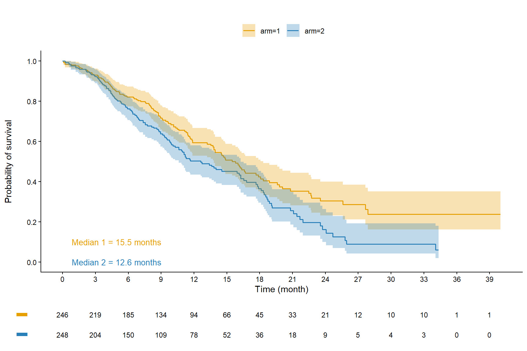
# Plot
fit <- survfit(Surv(time, event)~arm, data=data_ipd)

plot.CourbSurv <- ggsurvplot(fit, conf.int=TRUE,
                             xlab="Time (month)",
                             ylab="Probability of survival",
                             break.time.by=3, break.y.by = 0.2,
                             lwd=0.6, title="",
                             legend="top", legend.title="",
                             #legend.labs=c("Arm 1","Arm 2"),
                             palette=c("#E69F00","#2980B9"),
                             censor = FALSE,
                             ggtheme=theme_classic(),
                             risk.table=TRUE,
                             risk.table.title="Number at risk",
                             risk.table.y.text=FALSE,
                             risk.table.fontsize=3,
                             tables.theme=theme_cleantable())
plot.CourbSurv$plot <- plot.CourbSurv$plot +
  annotate("text", x=0, y=0.1, hjust=-0.1, size=3.5, color="#E69F00",
           label=paste0("Median 1 = ", round(surv_median(fit)$median,1)[1], " months")) +
  annotate("text", x=0, y=0, hjust=-0.1, size=3.5, color="#2980B9",
           label=paste0("Median 2 = ", round(surv_median(fit)$median,1)[2], " months"))
plot.CourbSurv$table <- plot.CourbSurv$table + theme(plot.title = element_blank())

ggarrange(plot.CourbSurv$plot, plot.CourbSurv$table, ncol = 1, nrow = 2, heights = c(0.85, 0.15), align = "v")

Step 1: Digitization

Step 2: Number at risk

Step 3: Pseudo individual patient data

Contact