The ggplot2 library allows to make a barplot using
geom_bar() with different options.
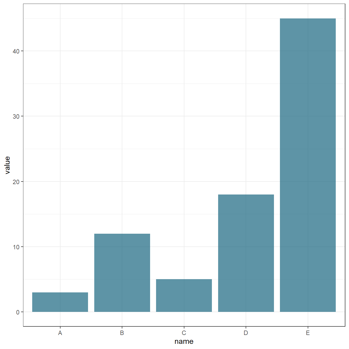
Barplot with stat = "identity"
With stat = "identity", you have to specify a
categorical variable for the X axis and a quantitative variable for the
Y axis. In this case, the bars are not automatically counted or
aggregated, instead, they directly reflect the values you supply in the
Y variable.
# Libraries
library(ggplot2)

# Creation of dataset
data <- data.frame(
  name=c("A","B","C","D","E") ,
  value=c(3,12,5,18,45)
  )

# A really basic barplot
ggplot(data, aes(x=name, y=value)) +
  geom_bar(stat = "identity", position = "identity",
           fill=rgb(0.1,0.4,0.5,0.7)) +
  theme_bw()
Different types of barplot can be created:
# Libraries
library(viridis)
library(ggplot2)
library(hrbrthemes)
library(tidyverse)
# Creation of dataset
data <- data.frame(
name = rep(c("A", "B", "C", "D"), each = 6),
time = rep(rep(c("M1", "M3"), each = 3), times = 4),
cat = rep(c("cat1", "cat2", "cat3"), times = 8),
value = c(3, 4, 12, 6, 5, 7, 18, 8,
7, 7, 11, 3, 10, 6, 5, 5,
7, 8, 3, 5, 5, 3, 15, 3)
)
# Basic barplot
ggplot(data, aes(x = name, y = value, fill = cat)) +
geom_bar(stat = "identity", position = "dodge") +
ggtitle("Basic barplot- Position: dodge") +
xlab("") +
theme_bw() +
theme(plot.title = element_text(size=11))
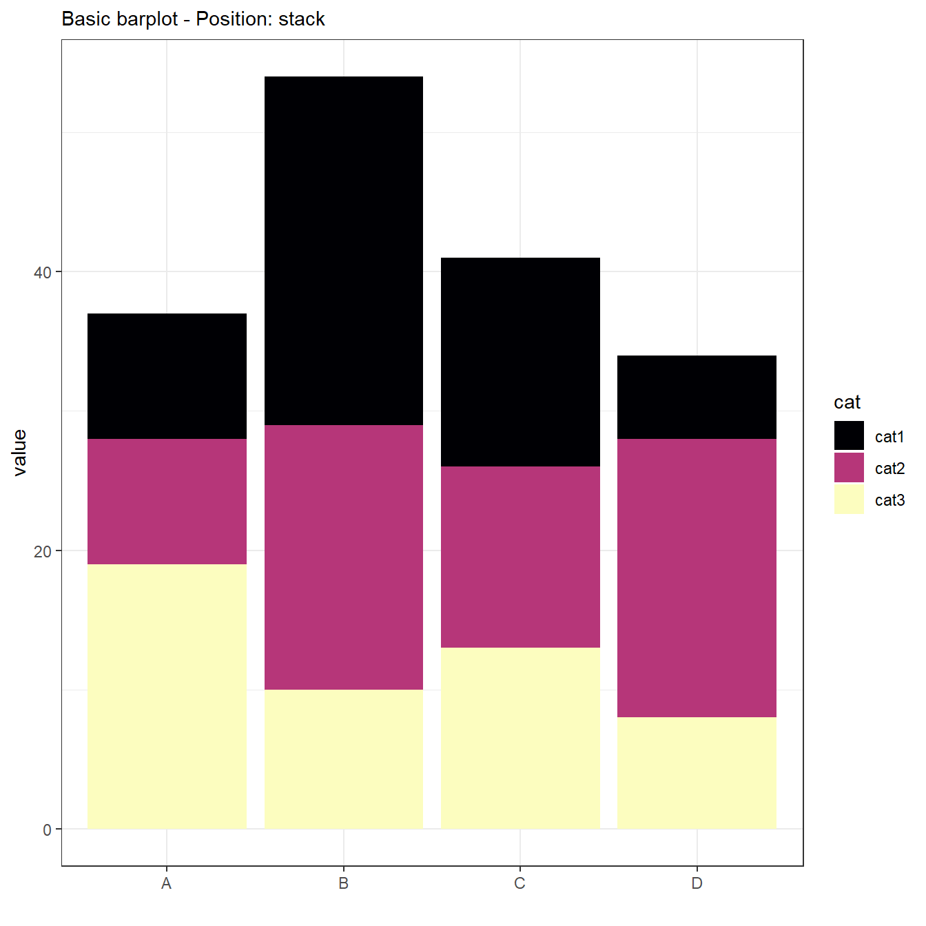
ggplot(data, aes(x = name, y = value, fill = cat)) +
geom_bar(stat = "identity", position = "stack") +
scale_fill_viridis(discrete = TRUE, option="A") +
theme_ipsum() +
ggtitle("Basic barplot - Position: stack") +
xlab("") +
theme_bw() +
theme(plot.title = element_text(size=11))
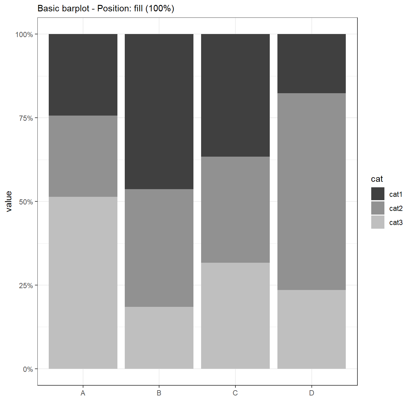
ggplot(data, aes(x = name, y = value, fill = cat)) +
geom_bar(stat = "identity", position = "fill") +
scale_fill_grey(start = 0.25, end = 0.75) +
ggtitle("Basic barplot - Position: fill (100%)") +
xlab("") +
scale_y_continuous(labels = scales::percent) +
theme_bw() +
theme(plot.title = element_text(size=11))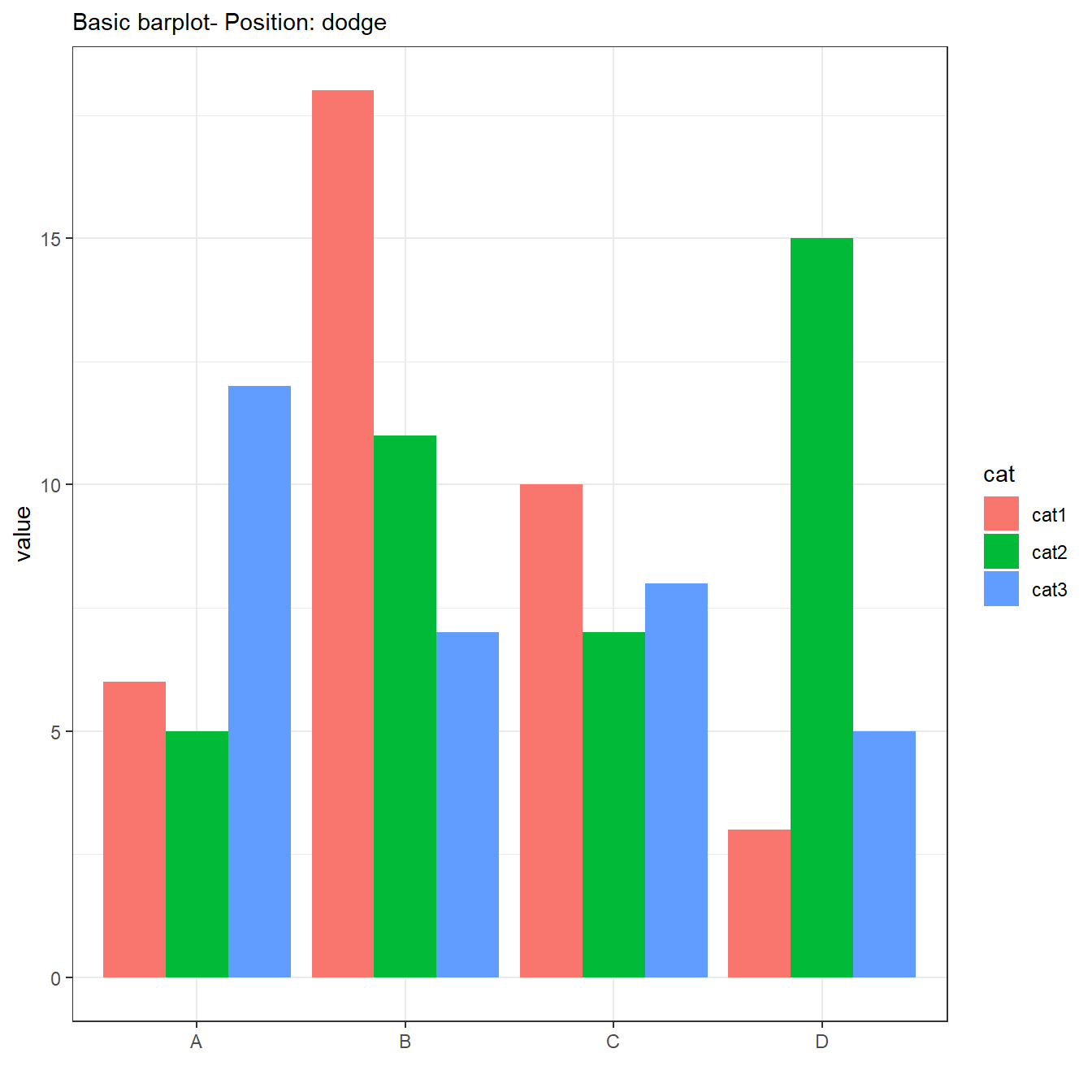
# Advanced barplot
ggplot(data, aes(x = name, y = value, fill = cat)) +
geom_bar(stat = "identity", position = "dodge") +
facet_wrap(~ time) +
ggtitle("Advanced barplot- Position: dodge") +
xlab("") +
theme_bw() +
theme(plot.title = element_text(size=11))
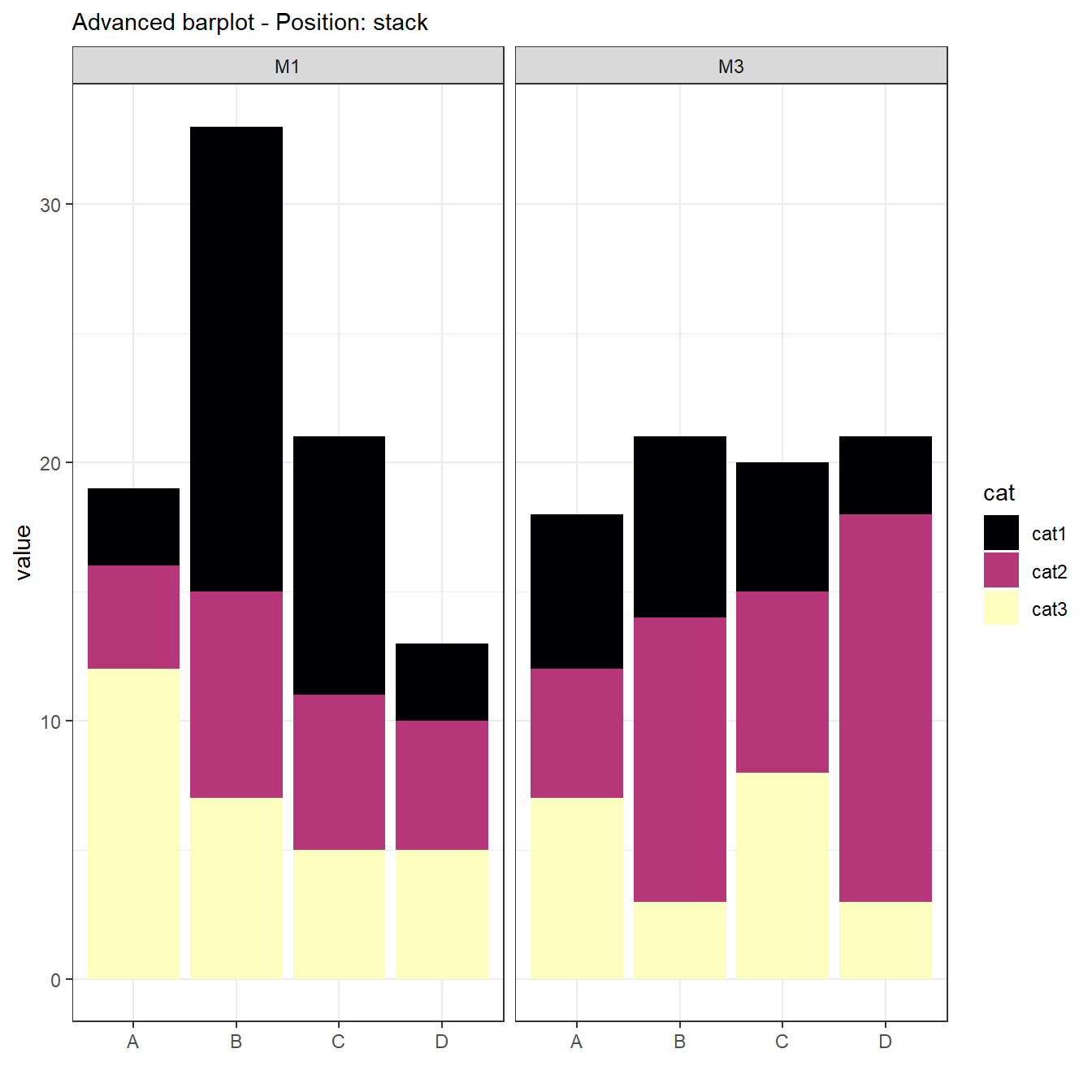
ggplot(data, aes(x = name, y = value, fill = cat)) +
geom_bar(stat = "identity", position = "stack") +
facet_wrap(~ time) +
scale_fill_viridis(discrete = TRUE, option="A") +
theme_ipsum() +
ggtitle("Advanced barplot - Position: stack") +
xlab("") +
theme_bw() +
theme(plot.title = element_text(size=11))
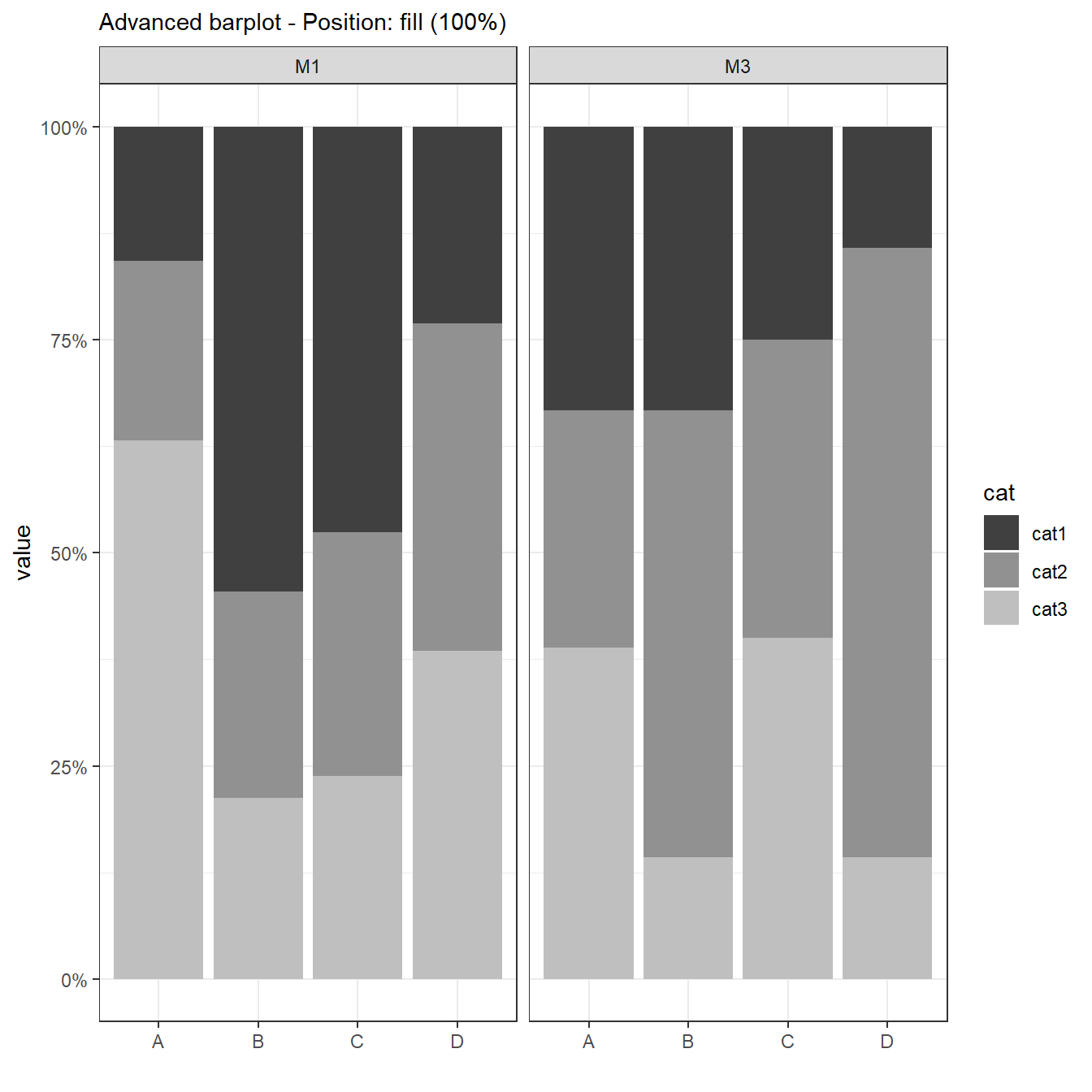
ggplot(data, aes(x = name, y = value, fill = cat)) +
geom_bar(stat = "identity", position = "fill") +
facet_wrap(~ time) +
scale_fill_grey(start = 0.25, end = 0.75) +
ggtitle("Advanced barplot - Position: fill (100%)") +
xlab("") +
scale_y_continuous(labels = scales::percent) +
theme_bw() +
theme(plot.title = element_text(size=11))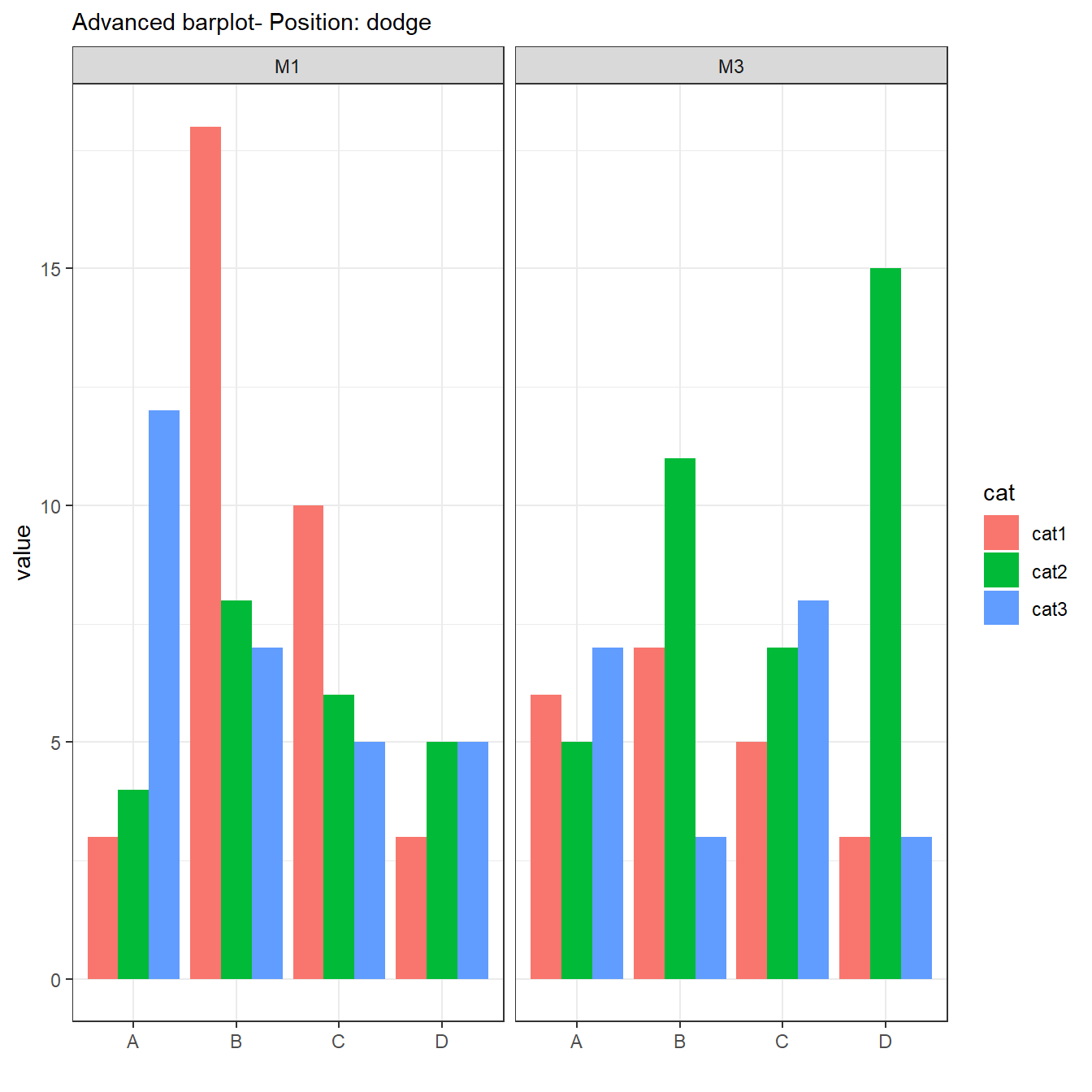
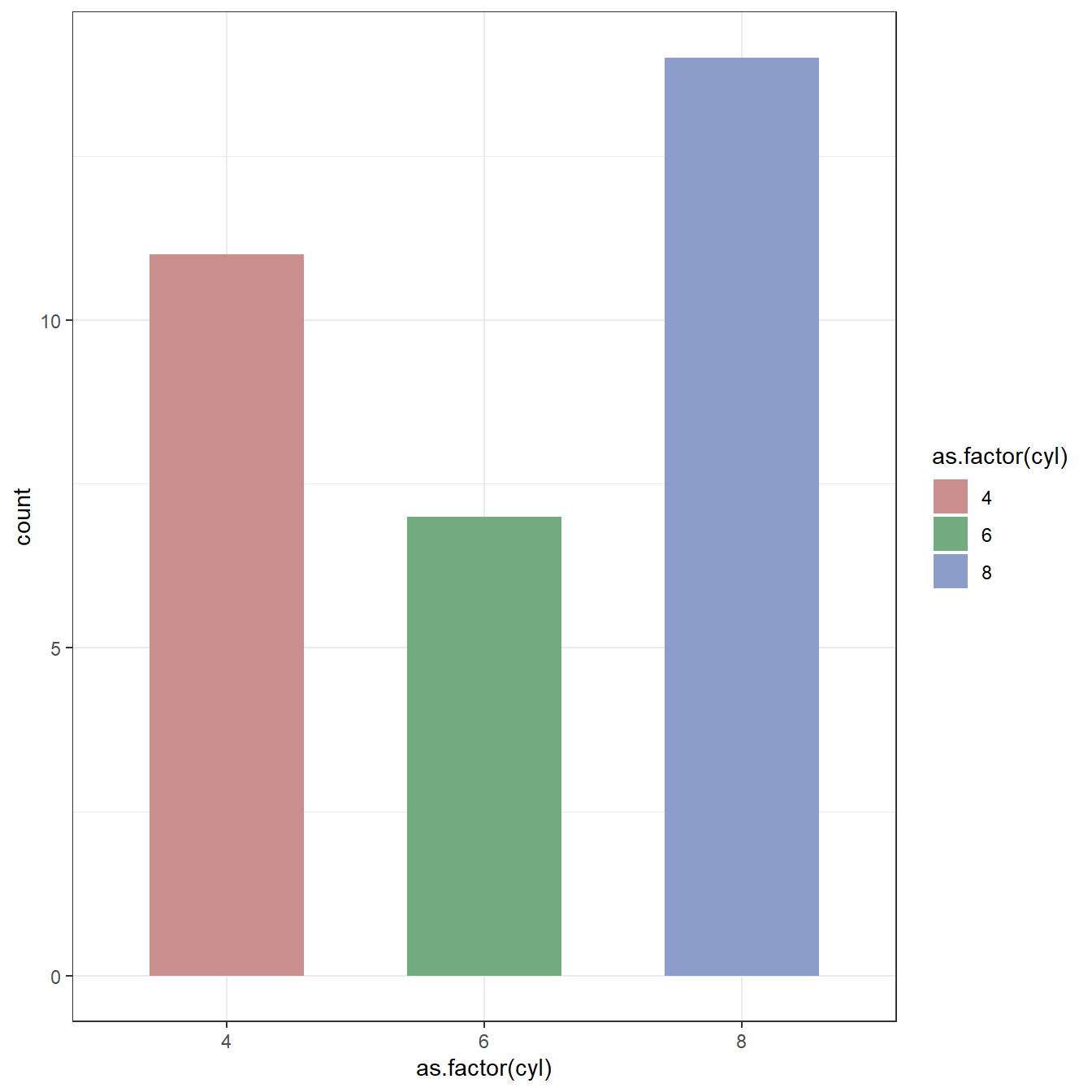
Barplot with stat = "count"
With stat = "count" (default behavior for
geom_bar()), you have to specify only a categorical
variable for the X axis, the Y values are calculated automatically. In
this case, the number of observations in each category are automatically
counted, and the height of each bar represents the number of rows with
that X value.
# Libraries
library(ggplot2)

# The mtcars dataset is natively available
# head(mtcars)

# A really basic barplot
ggplot(mtcars, aes(x=as.factor(cyl), fill=as.factor(cyl))) +
  geom_bar(stat = "count", position="identity", width=0.6) +
  scale_fill_hue(c = 40) +
  theme(legend.position="none") +
  theme_bw()
Different types of barplot can be created:
# Libraries
library(viridis)
library(ggplot2)
library(hrbrthemes)
library(tidyverse)
# Creation of dataset
set.seed(123)
data <- data.frame(
name=c( rep("A",500), rep("B",500), rep("C",20), rep('D', 100) ),
time=c( rep(c("M1", "M3"), each=250), rep(c("M1", "M3"), each=250), rep(c("M1", "M3"), each=10), rep(c("M1", "M3"), each=50) ),
cat=c( sample(c("cat1","cat2","cat3"), 500, replace=T),
sample(c("cat1","cat2","cat3"), 500, replace=T),
sample(c("cat1","cat2","cat3"), 20, replace=T),
sample(c("cat1","cat2","cat3"), 100, replace=T) )
)
# Basic barplot
ggplot(data, aes(x = name, fill = cat)) +
geom_bar(stat = "count", position = "dodge") +
ggtitle("Basic barplot- Position: dodge") +
xlab("") +
theme_bw() +
theme(plot.title = element_text(size=11))
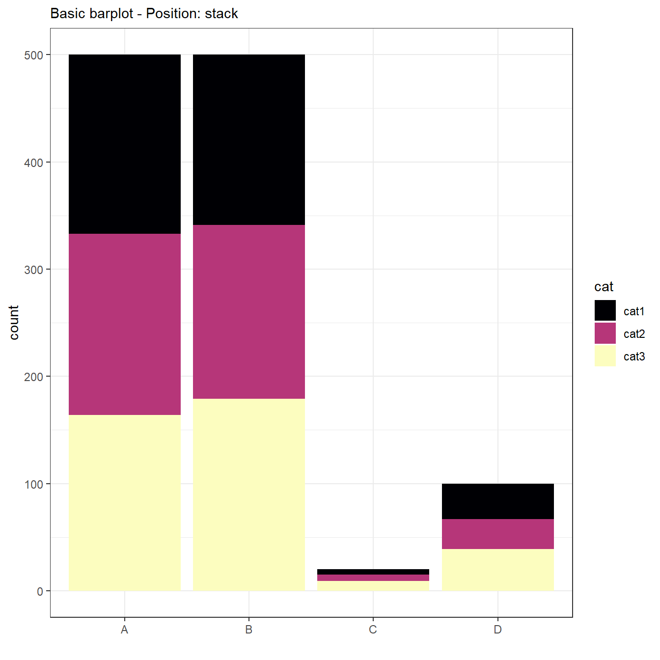
ggplot(data, aes(x = name,, fill = cat)) +
geom_bar(stat = "count", position = "stack") +
scale_fill_viridis(discrete = TRUE, option="A") +
theme_ipsum() +
ggtitle("Basic barplot - Position: stack") +
xlab("") +
theme_bw() +
theme(plot.title = element_text(size=11))
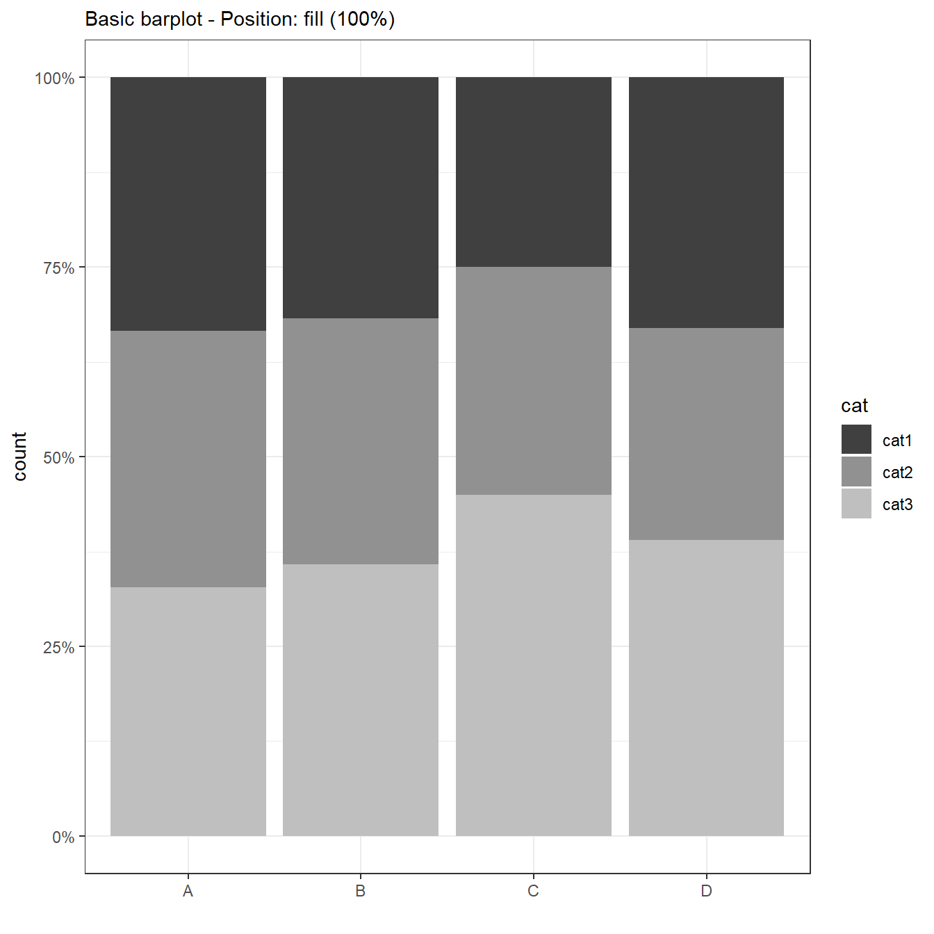
ggplot(data, aes(x = name, fill = cat)) +
geom_bar(stat = "count", position = "fill") +
scale_fill_grey(start = 0.25, end = 0.75) +
ggtitle("Basic barplot - Position: fill (100%)") +
xlab("") +
scale_y_continuous(labels = scales::percent) +
theme_bw() +
theme(plot.title = element_text(size=11))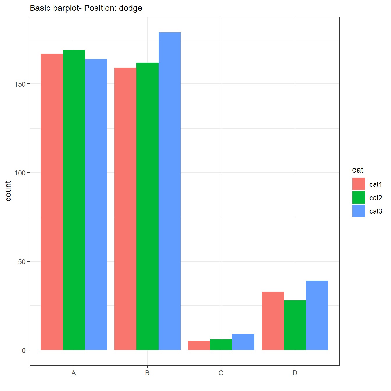
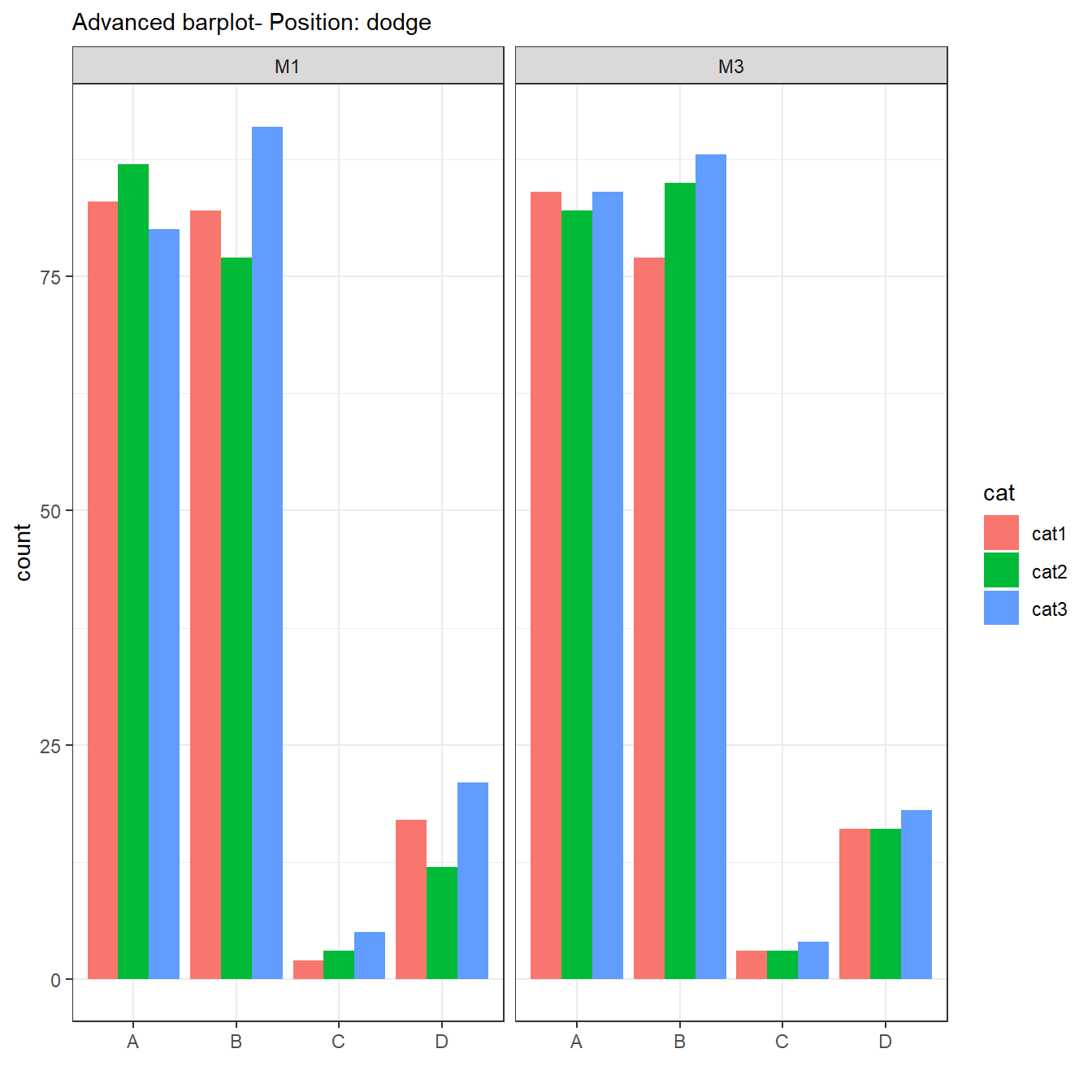
# Advanced barplot
ggplot(data, aes(x = name, fill = cat)) +
geom_bar(stat = "count", position = "dodge") +
facet_wrap(~ time) +
ggtitle("Advanced barplot- Position: dodge") +
xlab("") +
theme_bw() +
theme(plot.title = element_text(size=11))
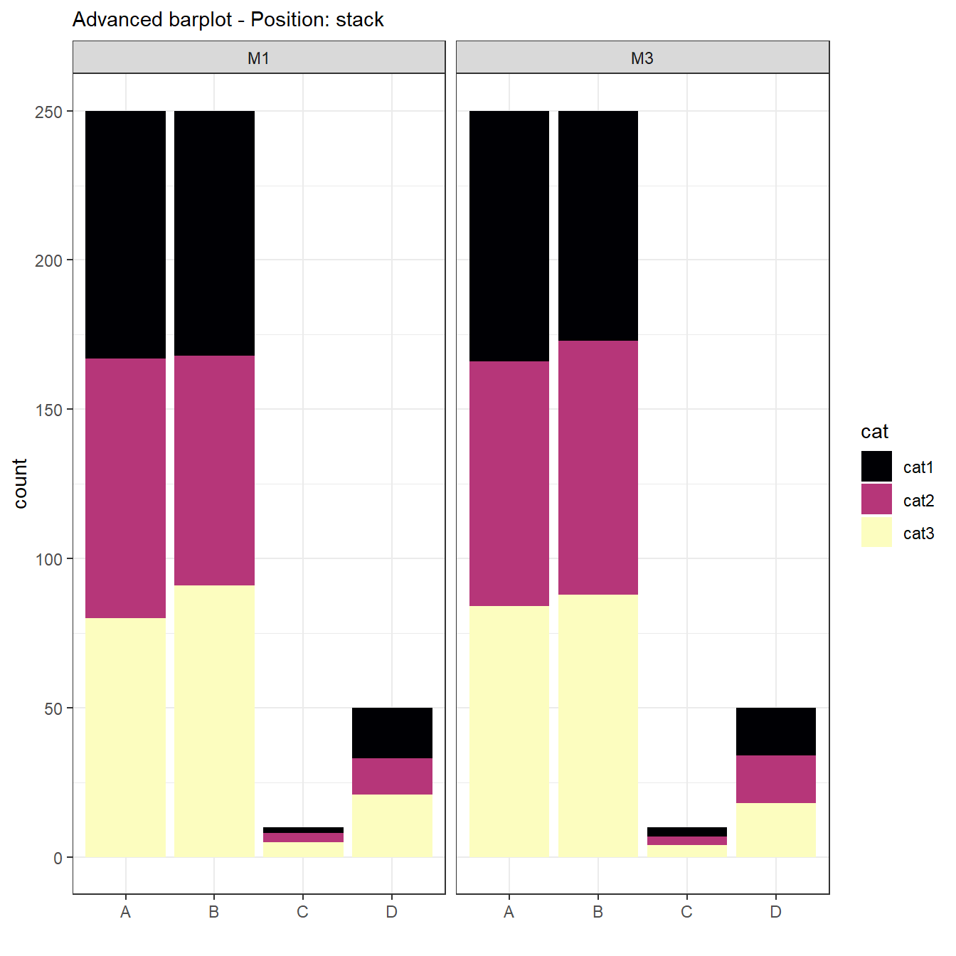
ggplot(data, aes(x = name, fill = cat)) +
geom_bar(stat = "count", position = "stack") +
facet_wrap(~ time) +
scale_fill_viridis(discrete = TRUE, option="A") +
theme_ipsum() +
ggtitle("Advanced barplot - Position: stack") +
xlab("") +
theme_bw() +
theme(plot.title = element_text(size=11))
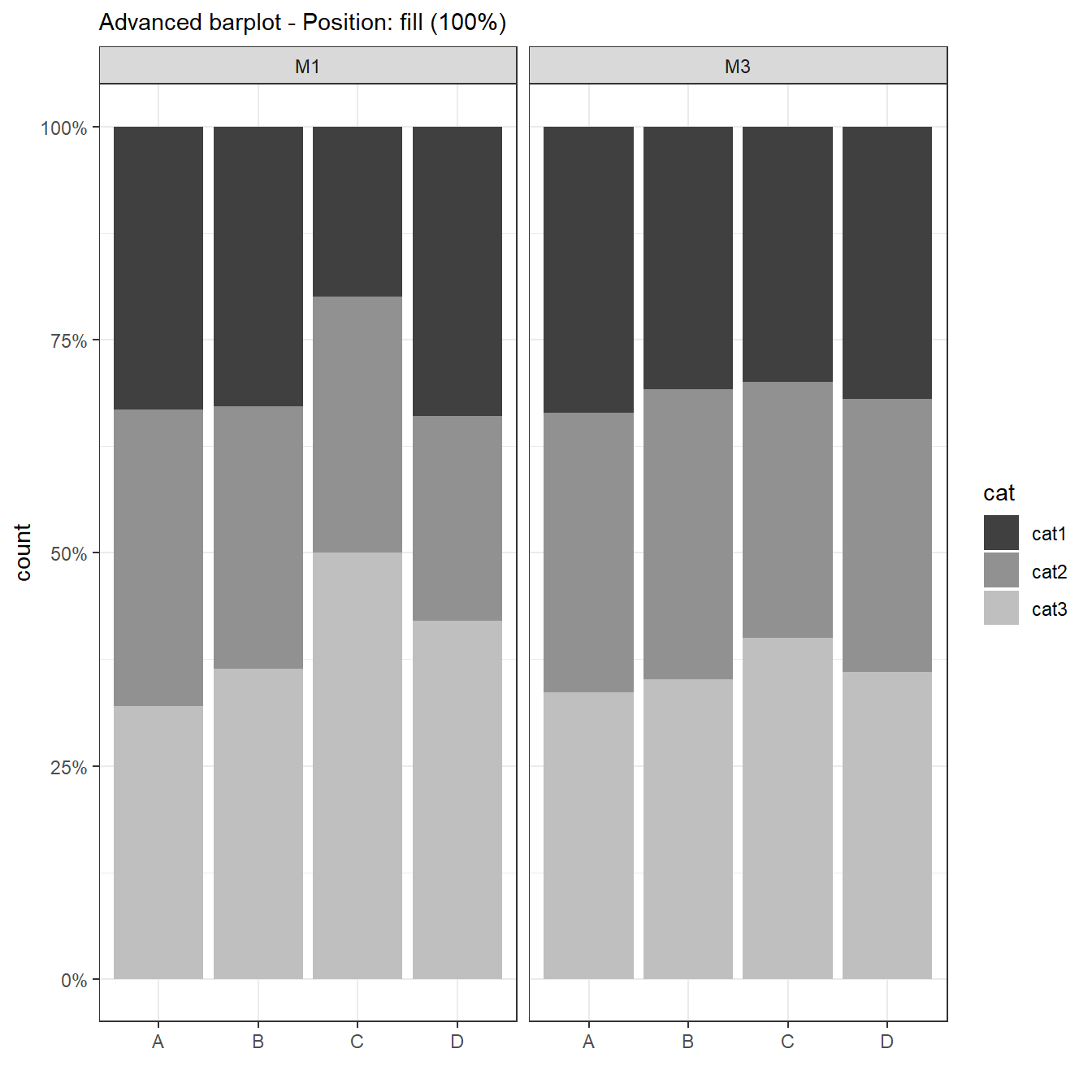
ggplot(data, aes(x = name, fill = cat)) +
geom_bar(stat = "count", position = "fill") +
facet_wrap(~ time) +
scale_fill_grey(start = 0.25, end = 0.75) +
ggtitle("Advanced barplot - Position: fill (100%)") +
xlab("") +
scale_y_continuous(labels = scales::percent) +
theme_bw() +
theme(plot.title = element_text(size=11))