Data
We build the following dataset:
# Creation of dataset
data <- data.frame(
  Evaluable=c(1,1,1,1,1,1,1,1,1,1,1,1,1,1,1,1,1,1,1,1,1,1,0,1),
  Therapy_Start_Date=c("2014-11-05", "2014-11-24", "2014-12-17", "2015-01-21", "2015-03-08",
                       "2015-04-12", "2015-05-03", "2015-08-08", "2015-08-24", "2016-01-12",
                       "2016-02-02", "2016-02-22", "2016-03-09", "2016-03-28", "2016-06-06",
                       "2016-07-10", "2016-10-10", "2017-03-27", "2017-04-26", "2017-07-11",
                       "2017-07-27", "2017-08-15", "2017-09-10", "2017-09-27"),
  Dose_Level=c("2", "2", "3", "4", "4", "4", "5", "4", "4", "4", "4", "3",
               "4", "4", "3", "3", "3", "3", "3", "3", "3", "3", "3", "3"),
  Last_Assessment_Date=c("2014-12-29", "2015-01-19", "2015-02-10", "2015-03-10", "2015-04-19",
                         "2015-06-10", "2015-05-24", "2015-10-03", "2015-09-14", "2016-03-08",
                         "2016-02-21", "2016-04-12", "2016-03-23", "2016-05-23", "2016-07-21",
                         "2016-07-25", "2016-10-24", "2017-05-24", "2017-06-07", "2017-07-25",
                         "2017-07-27", "2017-09-25", "2017-11-07", "2017-10-24"),
  DLT=c("0", "0", "0", "0", "0", "0", "1", "0", "0", "0", "1", "1",
        "0", "0", "0", "1", "0", "0", "1", "1", "0", "1", "0", "1")
)

data$Dose_Level <- factor(data$Dose_Level, c(2, 3, 4, 5))
data$Therapy_Start_Date <- as.Date(data$Therapy_Start_Date)
data$Last_Assessment_Date <- as.Date(data$Last_Assessment_Date)

data <- data[order(data[, "Therapy_Start_Date"]), ]
data$ID <- 1:nrow(data)
data format:
A data frame with 24 observations on the following 6 variables:
ID A distinct number or character for each patient. ID
order should correspond to the entry time of the patient. Start from 1
to the last patient
Evaluable The evaluable variable
should indicate whether or not the patient is evaluable in the trial. It
should be 0 or 1 (1 = Evaluable) for each entry
Therapy_Start_Date This variable gives the start date of
treatment
Dose_Level The dose level variable can be a
numeric or character variable indicating the dose level each patient has
been assigned
Last_Assessment_Date This variable gives
the last date of treatment
DLT The toxicity variable
should indicate whether or not a patient experienced a dose-limiting
toxicity (DLT). It should be 0 or 1 (1 = DLT) for each entry
| Evaluable | Therapy_Start_Date | Dose_Level | Last_Assessment_Date | DLT | ID |
|---|---|---|---|---|---|
| 1 | 2014-11-05 | 2 | 2014-12-29 | 0 | 1 |
| 1 | 2014-11-24 | 2 | 2015-01-19 | 0 | 2 |
| 1 | 2014-12-17 | 3 | 2015-02-10 | 0 | 3 |
| 1 | 2015-01-21 | 4 | 2015-03-10 | 0 | 4 |
| 1 | 2015-03-08 | 4 | 2015-04-19 | 0 | 5 |
| 1 | 2015-04-12 | 4 | 2015-06-10 | 0 | 6 |
| 1 | 2015-05-03 | 5 | 2015-05-24 | 1 | 7 |
| 1 | 2015-08-08 | 4 | 2015-10-03 | 0 | 8 |
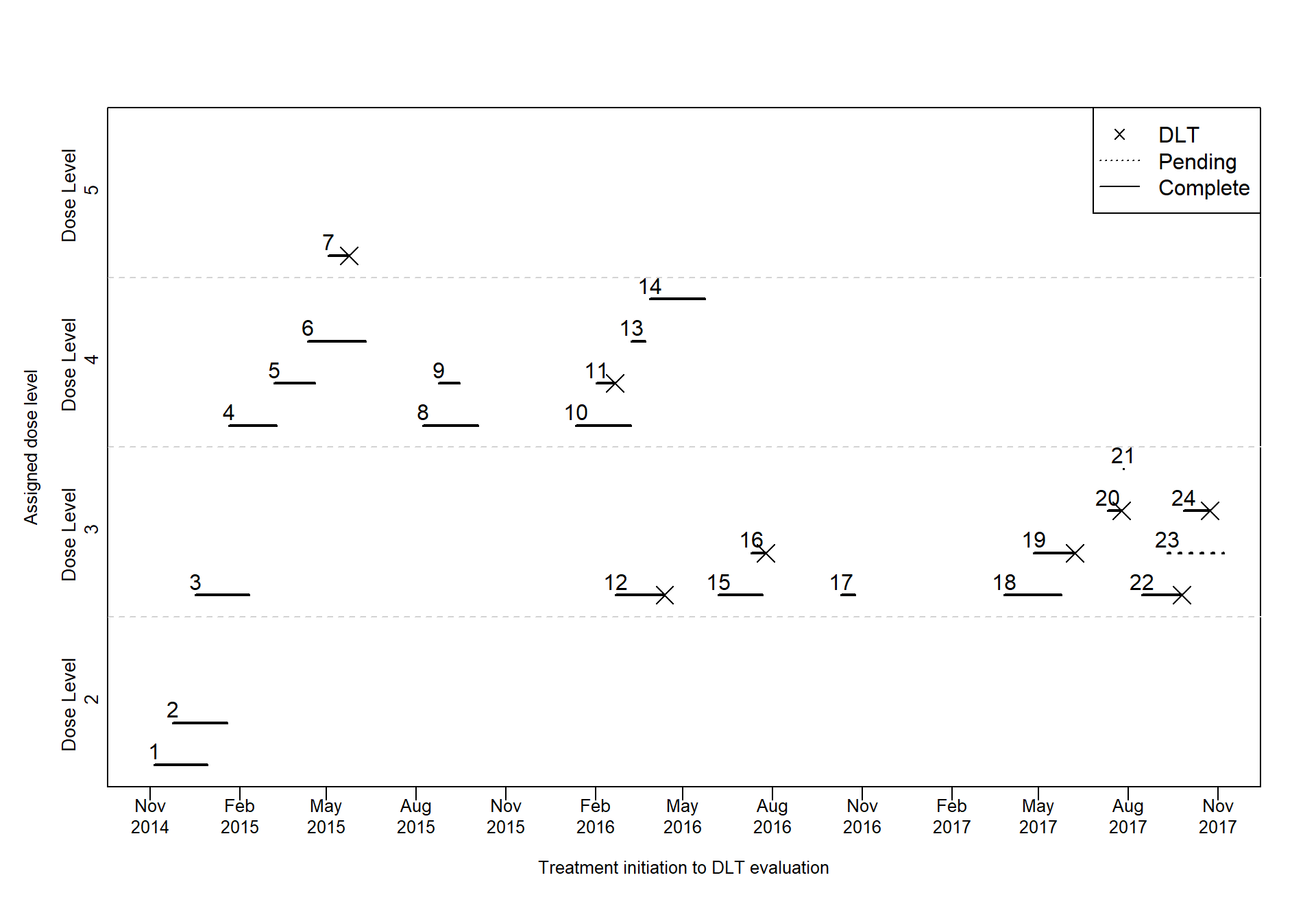
Piscine plot using base R
###### Parameters to be defined ######
# Sys.setlocale("LC_TIME", "fr_CA.UTF-8")
Sys.setlocale("LC_TIME", "en_US.UTF-8")

var_DLT <- "DLT"
var_Therapy_Start_Date <- "Therapy_Start_Date"
var_Last_Assessment_Date <- "Last_Assessment_Date"
var_Dose_Level <- "Dose_Level"
var_Evaluable <- "Evaluable"

n_obs <- 4 # how many observations do you want to have for each dose around the same time


###### Additional parameters ######
# `ID` A distinct number or character for each patient.
# ID order should correspond to the entry time of the patient. Start from 1 to the last patient
data <- data[order(data[, var_Therapy_Start_Date]), ]
data$ID <- 1:nrow(data)

vect_dose <- levels(data[, var_Dose_Level]) # dose counts
vect_dose_label <- sapply(vect_dose, function(x){paste0("Dose Level \n ",x)}) # y axis names for doses

symboles <- c(NA,4) # for DLT shape
linetype <- c(3, 1) # for pending or complete

data$y2 <- 0 # y2 is the new y coord for each patient
ymin <- 0.5; ymax <- 5.2 # the range of y axis (I don't think it's important)
ygap <- (ymax - ymin) / length(vect_dose) # the height for each dose in the plot

coord <- seq(ymin, ymax, ygap) # start and end coord for each dose category
y_coords <- list()
# the y coord for each observation around the same time (got from n_obs)
# let's say you want maximum of 4 obs around the same time, what are their coords?
for (i in 1:(length(coord)-1)) {
  ystart <- coord[i]
  yend <- coord[i+1]
  ymid <- seq(ystart + 0.15, yend - 0.15, length.out = n_obs)
  y_coords[[i]] <- ymid
}
names(y_coords) <- vect_dose_label
###### Piscine plot ######
cex <- 0.8
breaks <- seq(lubridate::floor_date(min(data[, var_Therapy_Start_Date]), unit = "months"),
lubridate::ceiling_date(max(data[, var_Last_Assessment_Date]), unit="months"), by="3 months")
# x11(width=9, height = 5)
plot(type="n",
x = c(min(breaks), max(breaks)), xlab="",
y = c(ymin, ymax), ylab="",
xaxt="n", yaxt="n",
tcl=-0.2, cex.lab=cex, cex.axis=cex,
cex=cex,lwd=1, yaxs = "i")
title(ylab="Assigned dose level",
xlab="Treatment initiation to DLT evaluation",
mgp=c(2.5,1,0), cex.lab=cex)
# axis(1, at = breaks, label=rep("", length(breaks)))
# text(x = breaks,
# y = par("usr")[3] - 0.2,
# labels = paste0(months(breaks, abbreviate = T), "./", stringr::str_sub(lubridate::year(breaks), 3, 4)),
# srt = 45,
# xpd = NA,
# # adj = 0.965,
# cex = cex)
axis(1, at = breaks, label=rep("", length(breaks)))
text(x = breaks,
y = par("usr")[3] - 0.2,
labels = paste0(format(breaks, "%b"),'\n',format(breaks, "%Y")),
xpd = NA,
# adj = 0.965,
cex = cex)
# lines dividing each dose category
abline(h=coord[-c(1, length(coord))], lty=2, col="lightgray")
# add y axis labels for each category
mtext(2, at=coord[-length(coord)]+ygap/2, line=0.2, text=vect_dose_label, las=0, cex=0.85)
# for each dose, calculate the
for (d in 1:length(vect_dose)){
test <- data[data[, var_Dose_Level] == vect_dose[d], ]
if (nrow(test) != 0){
count <- 0
y_test <- y_coords[[vect_dose_label[d]]]
for (i in 1:nrow(test)){
count <- count + 1
if (count > n_obs){
count <- 1
}
if (i != 1){
pre_end <- test[i-1, var_Last_Assessment_Date]
cur_start <- test[i, var_Therapy_Start_Date]
if (cur_start > (pre_end+ (max(data[, var_Last_Assessment_Date]) - min(data[, var_Therapy_Start_Date])) * 0.045)){
count <- 1
}
}
test$y2[i] <- y_test[count]
}
points(test[, var_Last_Assessment_Date], test$y2, pch = symboles[as.numeric(as.character(test[, var_DLT]))+1], cex = 1.8)
with(test, segments(get(var_Therapy_Start_Date), y2, get(var_Last_Assessment_Date), y2, lty = linetype[as.numeric(as.character(test[, var_Evaluable]))+1], lwd = 2))
text(test[, var_Therapy_Start_Date], test$y2 + ygap/(3*n_obs), test$ID, cex = 1)}
}
legend("topright", legend = c("DLT", "Pending", "Complete"),
lty = c(NA,3,1),
pch = c(symboles[2], NA, NA),
cex = 1)